You can add a colorbar to a graphic. Colorbars show the minimum to maximum pixel values on a color scale.
See the following sections:
Example: DEM
The following example shows a digital elevation model (DEM) taken from the Santa Monica mountains in California. The colors in the graphic are determined by the RGB_TABLE, which the COLORBAR function uses to create the color scale.
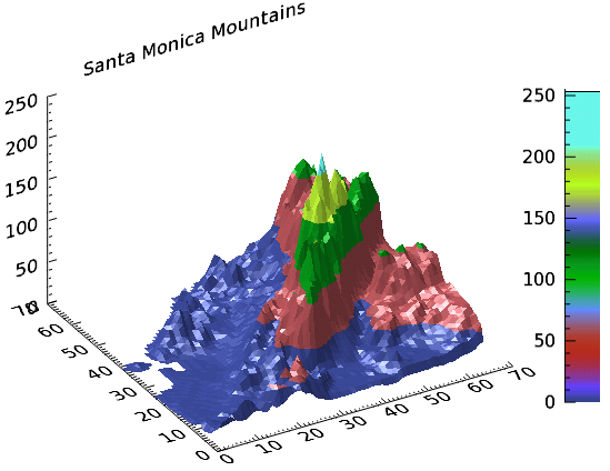
The code shown below creates the graphic shown above. You can copy the entire block and paste it into the IDL command line to run it.
file = FILE_WHICH('elevbin.dat')
dem = READ_BINARY(file, data_dims=[64,64])
c1 = CONTOUR(dem, $
RGB_TABLE=30, $
/FILL, $
PLANAR=0, $
TITLE='Santa Monica Mountains')
cbar = COLORBAR(TARGET = c1, ORIENTATION=1, $
POSITION=[0.90, 0.2, 0.95, 0.75])
(c1['zaxis']).location = [0, (c1.yrange)[1], 0]
Example: Discrete Contour Levels with Colorbar
You can display a colorbar that matches discrete contour levels.
The following example shows a simple contour image generated from the DIST function. The colors in the graphic are determined by the RGB_TABLE, which the COLORBAR function uses to create the color scale.
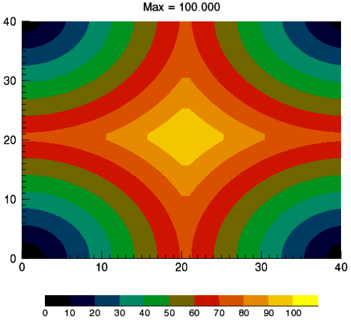
The code shown below creates the graphic shown above. You can copy the entire block and paste it into the IDL command line to run it.
d = DIST(41)
fmax = 100.0
f = d / max(d) * fmax
n_levels = 11
levels = FINDGEN(n_levels)/(n_levels-1)*fmax
ct_number = 4
ct_indices = BYTSCL(levels)
LOADCT, ct_number, RGB_TABLE=ct, /SILENT
step_ct = CONGRID(ct[ct_indices, *], 256, 3)
; interpolated indices.
c1 = CONTOUR(f, $
c_value = levels, $
RGB_TABLE = step_ct, $
RGB_INDICES = ct_indices, $
/FILL, $
MARGIN = [0.15, 0.20, 0.15, 0.15], $
TITLE = 'Max = ' + strtrim(fmax,2), $
WINDOW_TITLE = 'Discrete Colorbar Example')
tick_labels = [STRTRIM(FIX(levels), 2), '']
cb = COLORBAR( $
TARGET = c1, $
TICKLEN = 0, $
MAJOR = n_levels+1, $
TICKNAME = tick_labels, $
FONT_SIZE = 10, $
POSITION = [0.2, 0.07, 0.8, 0.1])
Example: Two Contour Plots with One Colorbar
The following example shows two simple contour images generated from the DIST function, annotated with one colorbar.
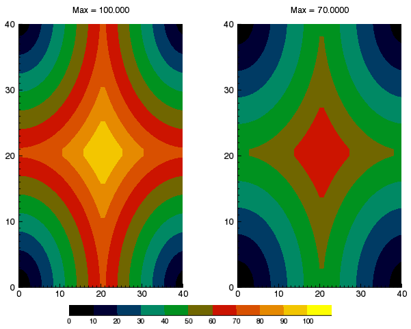
The code shown below creates the graphic shown above. You can copy the entire block and paste it into the IDL command line to run it.
d = DIST(41)
max1 = 100.0
max2 = 70.0
f1 = d / max(d) * max1
f2 = d / max(d) * max2
n_levels = 11
levels = FINDGEN(n_levels)/(n_levels-1)*max1
ct_number = 4
ct_indices = BYTSCL(levels)
LOADCT, ct_number, RGB_TABLE = ct, /SILENT
step_ct = CONGRID(ct[ct_indices, *], 256, 3)
c1 = CONTOUR(f1, $
LAYOUT = [2,1,1], $
C_VALUE = levels, $
RGB_TABLE = step_ct, $
RGB_INDICES = ct_indices, $
/FILL, $
TITLE = 'Max = ' + strtrim(max1,2), $
WINDOW_TITLE = 'Discrete Colorbar Example')
c2 = CONTOUR(f2, $
LAYOUT = [2,1,2], $
/CURRENT, $
C_VALUE = levels, $
RGB_TABLE = ct_number, $
RGB_INDICES = ct_indices, $
/FILL, $
TITLE = 'Max = ' + strtrim(max2,2))
tick_labels = [STRTRIM(FIX(levels), 2), '']
cb = COLORBAR( $
TARGET = c1, $
TICKLEN = 0, $
MAJOR = n_levels+1, $
TICKNAME = tick_labels, $
FONT_SIZE = 8, $
POSITION = [0.2, 0.06, 0.8, 0.09])
Properties used in the examples
CONTOUR
- RGB_TABLE - defines the color table used to display the image. COLORBAR uses the colors defined in this property.
- FILL - specifies that the contour is filled. This keyword uses the colors defined in RGB_TABLE.
- PLANAR - PLANAR = 0 displays the graphic in three-dimensional space rather than on a plane. The default is PLANAR=1, which displays a graphic on a plane.
- TITLE - defines the title of the view rather than the graphic.
COLORBAR
- ORIENTATION - ORIENTATION =1 defines a vertical colorbar direction. The default orientation is 0, which is horizontal.
- POSITION - defines the location of the colorbar in a four-element vector: [X1, Y1, X2, Y2], defining the lower left and upper right corners of the image portion of the colorbar.
Resources