Part of the project in this study area involved characterizing both the current extent of the tritium plume and predicting its future extent. The file "MonitoringWells.csv" contains data from current readings of tritium concentrations (T0) as well as three future states modeled using separate algorithms. For this example, use the data for column T3 which corresponds to the plume extent for 2030.
Create Contour Plot of Tritium Plume Future State
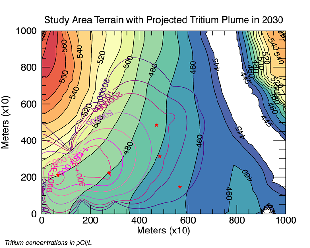
Using the data in the files "MonitoringWells.csv" and "TankTerrainData.csv", create a contour plot over the top of the terrain to display the calculated extent of the tritium plume in 2030. Note that the solid white area in the upper right denotes the extent of the river at the 445 m contour.
Copy the code examples below to your IDL command line to create a graphic similar to this:
Read In and Grid the Terrain and Plume Data
Start by reading in the terrain and plume data files. The terrain data resides in the TankTerrainData.csv file in the \examples\data directory of your IDL installation. This data contains the surface terrain of our site in X, Y, Z coordinates (all in meters), and the fourth column contains the elevation of the surface of the underlying aquifer. The second file ("MonitoringWells.csv") contains the concentrations of tritium over the study area at four different times (T0=current, T1=2020, T2=2025, T3=2030).
In this example, we create templates using ASCII_TEMPLATE, then read in the data using READ_ASCII.
myTemplate = ASCII_TEMPLATE()
site = READ_ASCII('TankDataTerrain.csv', $
TEMPLATE=myTemplate)
grid = GRIDDATA(site.X, site.Y, site.Z, $
DIMENSION=1000, METHOD="Kriging")
myTemplate2 = ASCII_TEMPLATE()
wells = READ_ASCII('MonitoringWells.csv', $
TEMPLATE=myTemplate2)
gridT3 = GRIDDATA(wells.X, wells.Y, wells.T3, $
DIMENSION=1000, METHOD="Kriging")
Create the Base Contour Map
Create the base contour plot. We will then overplot with the tritium plume contours, and later use SCATTERPLOT to indicate the tank locations.
Note that starting the index contour values at 445 coincides with the level of the river and will show up as white in the resulting map.
myCT = COLORTABLE(74, /REVERSE)
index = [445,450,460,470,480,490,500,510,520,530, $
540,550,560,570,580]
myContour = CONTOUR(grid, RGB_TABLE=myCT, $
C_VALUE=index, ASPECT_RATIO=.75, /FILL, $
TITLE="Study Area Terrain with Tank Locations", $
XTITLE="Meters (x10)", YTITLE="Meters (x10)")
myContour2 = CONTOUR(grid, COLOR='black', $
C_VALUE=index, ASPECT_RATIO=.75, /OVERPLOT)
Create the Tritium Contours with Well Locations
Create the plot of simulated tritium plume extent for T3 (2030).
xLoc = [66,276,566,471,484]
yLoc = [210,221,146,483,313]
colors = ['indigo','purple','medium violet red','medium orchid', $
'hot pink','fuchsia','deep pink']
index2 = [20000,100000,200000,500000,1000000,1500000,2000000]
myContourT3 = CONTOUR(gridT3, ASPECT_RATIO=.75, C_LABEL_INTERVAL=0.75, $
C_VALUE=index2, C_LABEL_SHOW=1, C_COLOR=colors, /OVERPLOT)
areaText2 = TEXT(-.15, -.17, TARGET=myContourB, /RELATIVE, $
'Tritium concentrations in pCi/L', $
COLOR='black', FONT_SIZE=8, FONT_STYLE='italic')
tanks = SCATTERPLOT(xLoc, yLoc, /SYM_FILLED, SYMBOL='star', $
SYM_COLOR='red', /OVERPLOT, /DATA)
Other Topics in this Series
See Also
ASCII_TEMPLATE, COLORTABLE, CONTOUR, GRIDDATA, READ_ASCII, READ_CSV, SCATTERPLOT, TEXT