IMSL_BSINTERP

The IMSL_BSINTERP function computes a one- or two-dimensional spline interpolant.

This routine requires an IDL Advanced Math and Stats license. For more information, contact your sales or technical support representative.

The IMSL_BSINTERP function is designed to compute either a one-dimensional spline interpolant or two-dimensional, tensor-product spline interpolant to input data. The decision of whether to compute the one- or two-dimensional spline is based on the number of arguments passed to the function. Keywords are provided to allow the user to specify the order of the spline and the knots used for the spline. When computing a one-dimensional spline, the available keywords are XORDER and XKNOTS. When computing a two-dimensional spline, the order and knots in x-direction and/or y-direction can be specified using the keywords XORDER, XKNOTS, YORDER, and YKNOTS.

Separate discussions on one- and two-dimensional splines follow.

One-dimensional B-splines

Given the data points x = Xdata, f = Fdata, and the number of elements (n) in Xdata and Fdata, the default action of IMSL_BSINTERP computes a cubic (k = 4) spline interpolant s to the data using the default knot sequence generated by the IMSL_BSKNOTS function.

Optional keyword XORDER allows the user to choose the order, k, of the spline interpolant; optional keyword XKNOTS allows user specification of knots.

The IMSL_BSINTERP function is based on the routine SPLINT by de Boor (1978, p. 204).

First, IMSL_BSINTERP sorts the Xdata vector and stores the result in x. The elements of the Fdata vector are permuted appropriately and stored in f, yielding the equivalent data (x_i, f_i) for i = 0 to n -1.

The following preliminary checks are performed on the data:

x_i < x_i _{+ 1} i = 0, ..., n - 2

t_i < t_{i + k} i = 0, ..., n – 1

t_t £ t_{i + 1} i = 0, ..., n + k - 2

The first test checks to see that the abscissas are distinct. The second and third inequalities verify that a valid knot sequence has been specified.

In order for the interpolation matrix to be nonsingular, t_k_{– 1} £ x_i ≤ t_nis also checked for i = 0 to n - 1. This first inequality in the last check is necessary since the method used to generate the entries of the interpolation matrix requires that the k possibly nonzero B-splines at x_i:

B_{j – k +}₁, ..., B_j where j satisfies t_j ≤ x_i < t_{j +}₁

be well-defined (that is, j – k + 1 ≥ 0).

General conditions are not known for the exact behavior of the error in spline interpolation; however, if t and x are selected properly and the data points arise from the values of a smooth (for example, C^k) function f, i.e., fi = f(xi), then the error behaves in a predictable fashion. The maximum absolute error satisfies:

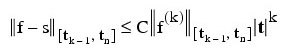
where the following is true:

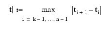
For more information on this, see de Boor (1978, Chapter 13) and the references therein. This function can be used in place of the IMSL_CSINTERP function.

The returned value for this function is a structure. This structure contains all the information to determine the spline (stored as a linear combination of B-splines) that is computed by this function. For example, the following code sequence evaluates this spline at x and returns the value in y:

y = IMSL_SPVALUE(x, spline)

Two-dimensional, Tensor-product B-splines

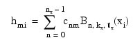
If arguments xdata, ydata, and fdata are all included in the call to the IMSL_BSINTERP function, the function computes a two-dimensional, tensor-product spline interpolant. The tensor-product spline interpolant to data {(x_i, y_j, f_ij)}, where 0 ≤ i ≤ n_x – 1 and 0 ≤ j ≤ n_y - 1, has the form:

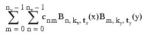
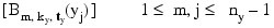
where k_x and k_y are the orders of the splines. These numbers are defaulted to 4 but can be set to any positive integer using keywords XORDER and YORDER. Likewise, t_x and t_y are the corresponding knot sequences (XKNOTS and YKNOTS). These values are defaulted to the knots returned by the IMSL_BSKNOTS function. The algorithm requires that the following is true:

t_x (k_x – 1) ≤ x_i ≤ t_x (n_x) 0 ≤ i ≤ n_x – 1

t_y (k_y – 1) ≤ y_j≤ t_y (n_y) 0 ≤ j ≤ n_y - 1

Tensor-product spline interpolants in two dimensions can be computed quite efficiently by solving (repeatedly) two univariate interpolation problems. The computation is motivated by the following observations:

Setting:

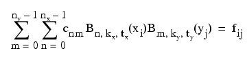
Note that for each fixed i from 0 to n_x – 1, there are n_y linear equations in the same number of unknowns as can be seen below:

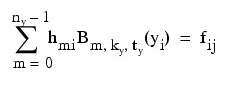
The same matrix appears in the previous equation.

Thus, this matrix is factored only once, then the factorization to solve the n_x right-hand sides is applied. Once this is done and h_mi is computed, then the coefficients c_nm are solved using the relation:

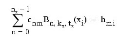
for m from 0 to n_y – 1, which involves one factorization and n_y solutions to the different right-hand sides. This ability of the IMSL_BSINTERP function is based on the SPLI2D routine by de Boor (1978, p. 347).

The returned value is a structure containing all the information to determine the spline (stored in B-spline format) that is computed by this function. For example, the following code sequence evaluates this spline at (x, y) and returns the value in z:

z = IMSL_SPVALUE(x, y, spline)

Examples

Example 1

In this example, a one-dimensional B-spline interpolant to function values is computed, as shown in the figure that follows. Evaluations of the computed spline are then plotted along with the original data values. Since the default settings are being used, the interpolant is determined by the not-a-knot condition (see de Boor 1978).

x = FINDGEN(11)/10

; Define data values. f = SIN(15 * x)

bs = IMSL_BSINTERP(x, f)

; Compute interpolant.

bsval = IMSL_SPVALUE(FINDGEN(100)/99, bs) PLOT, FINDGEN(100)/99, bsval

; Output results. OPLOT, x, f, Psym = 6

Example 2

In this example, a two-dimensional, tensor-product B-spline interpolant to gridded data is computed as shown in the figure that follows.

x = FINDGEN(5)/4

; Define the abscissas in the x-direction.

y = FINDGEN(5)/4

; Define the abscissas in the y-direction.

f = FLTARR(5, 5)

; Define the sample function values.

FOR i = 0, 4 DO $

  f(i, *) = SIN(2 * x(i)) - COS(5 * y)

bs = IMSL_BSINTERP(x, y, f)

; Compute the spline interpolant.

bsval = IMSL_SPVALUE(FINDGEN(20)/19, FINDGEN(20)/19, bs)

; Use IMSL_SPVALUE to evaluate the computed spline.

!P.Charsize = 1.5

!P.Multi = [0, 1, 2]

WINDOW, XSize = 400, YSize = 800

; Plot the original and computed surfaces in a tall window.

SURFACE, f, x, y

SURFACE, bsval, FINDGEN(20)/19, $ FINDGEN(20)/19

Errors

Warning Errors

MATH_ILL_COND_INTERP_PROB: Interpolation matrix is ill-conditioned. Solution might not be accurate.

Fatal Errors

MATH_DUPLICATE_XDATA_VALUES: The Xdata values must be distinct.

MATH_YDATA_NOT_INCREASING: The Ydata values must be strictly increasing.

MATH_KNOT_MULTIPLICITY: Multiplicity of the knots cannot exceed the order of the spline.

MATH_KNOT_NOT_INCREASING: Knots must be nondecreasing.

MATH_KNOT_XDATA_INTERLACING: The i-th smallest element of Xdata (x_i) must satisfy t_i ≤ x_i < t_{i + Order}, where t is the knot sequence.

MATH_XDATA_TOO_LARGE: Array Xdata must satisfy Xdata_i ≤ t_ndata, for i = 1, ..., Ndata.

MATH_XDATA_TOO_SMALL: Array Xdata must satisfy Xdata_i ≤ t_ndata, for i = 1, ..., Ndata

MATH_KNOT_DATA_INTERLACING: The i-th smallest element of the data arrays Xdata and Ydata must satisfy t_i ≤ data_{i + Order}, where t is the knot sequence.

MATH_DATA_TOO_LARGE: Data arrays xdata and ydata must satisfy datai ≤ tnum_data, for i = 1, ..., num_data.

MATH_DATA_TOO_SMALL: Data arrays xdata and ydata must satisfy datai ≥ tOrder – 1, for i = 1, ..., num_data.

Syntax

Result = IMSL_BSINTERP(Xdata, Fdata [, /DOUBLE] [, XKNOTS=value] [, XORDER=value] [, YKNOTS=value] [, YORDER=value])

Result = IMSL_BSINTERP(Xdata, Ydata, Fdata [, DOUBLE=value] [, XKNOTS=value] [, XORDER=value] [, YKNOTS=value] [, YORDER=value])

Return Value

A structure containing information that defines the one- or two-dimensional spline.

Arguments

If a one-dimensional spline is desired, then the arguments Xdata and Fdata are required. If a two-dimensional, tensor-product spline is desired, then Xdata, Ydata, and Fdata are required.

Xdata

Array containing the abscissas in the x-direction of the interpolation problem.

Ydata

Array containing the abscissas in the y-direction of the interpolation problem.

Fdata

Array containing the ordinates of the interpolation problem. If a one-dimensional spline is being computed, then Fdata(i) is the data value at Xdata(i). If a two-dimensional spline is being computed, then Fdatais a two-dimensional array, where Fdata(i, j) is the data value at (Xdata(i), Ydata(i)).

Keywords

DOUBLE (optional)

If present and nonzero, then double precision is used.

XKNOTS (optional)

Specifies the array of knots in the x-direction to be used when computing the definition of the spline. Default: knots are selected by the IMSL_BSKNOTS function using its defaults.

XORDER (optional)

Specifies the order of the spline in the x-direction. Default: 4, i.e., cubic splines.

YKNOTS (optional)

Specifies the array of knots in the y-direction to be used when computing the definition of the spline. Default: knots are selected by the IMSL_BSKNOTS function using its defaults.

YORDER (optional)

Specifies the order of the spline in the y-direction. If a one-dimensional spline is being computed, then YORDER has no effect on the computations. Default: 4, i.e., cubic splines.

Version History

6.4	Introduced

Module	Math&Stats

Version	9.0