The IMSL_CAT_GLM function analyzes categorical data using logistic, Probit, Poisson, and other generalized linear models.
This routine requires an IDL Advanced Math and Stats license. For more information, contact your sales or technical support representative.
The IMSL_CAT_GLM function uses iteratively reweighted least squares to compute (extended) maximum likelihood estimates in some generalized linear models involving categorized data. One of several models, including the probit, logistic, Poisson, logarithmic, and negative binomial models, may be fit.
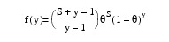
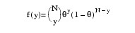
Note that each row vector in the data matrix can represent a single observation; or, through the use of keyword IFREQ, each row can represent several observations. Also note that classification variables and their products are easily incorporated into the models via the usual regression-type specifications. The models available in IMSL_CAT_GLM are listed in the following table.
|
Model |
PDF of the Response Variable
|
Parameterization
|
|
0 |
f(y) = (λyexp(-λ)) / y
|
λ = N x exp(ω + η)
|
|
1 |
|
|
|
2 |

|
|
|
3 |
|
|
|
4 |
|
θ = Φ (ω + η)
|
|
5 |
|
θ = 1 − exp (−exp (ω + η) )
|
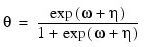
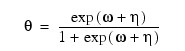
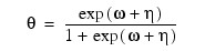
Here, Φ denotes the cumulative normal distribution. N and S are known distribution parameters specified for each observation via the keyword IPAR. ω is an optional fixed parameter of the linear response, γi, specified for each observation. (If the keyword IFIX is not used, then ω is taken to be 0.) Since the log-log model (Model = 5) probabilities are not symmetric with respect to 0.5, quantitatively, as well as qualitatively, different models result when the definitions of "success" and "failure" are interchanged in this distribution. In this model and all other models involving θ, θ is taken to be the probability of a "success".
Computational Details
The computations proceed as follows:
- The input parameters are checked for consistency and validity.
- Estimates of the means of the "independent" or design variables are computed. The frequency or the observation in all but binomial distribution models is taken from vector frequencies. In binomial distribution models, the frequency is taken as the product of n = parameter (i) and frequencies (i). Means are computed as:

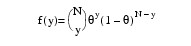
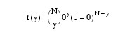
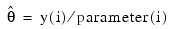
- By default, unless the keyword INIT_EST is used, initial estimates of the coefficients are obtained (based upon the observation intervals) as multiple regression estimates relating transformed observation probabilities to the observation design vector. For example, in the binomial distribution models, θ may be estimated as:
and, when Model=3, the linear relationship is given by:
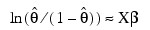
while, if Model = 4, Φ-1 (θ) = Xβ. When computing initial estimates, standard modifications are made to prevent illegal operations such as division by zero. Regression estimates are obtained at this point, as well as later, by use of IMSL_MULTIREGRESS.
- Newton-Raphson iteration for the maximum likelihood estimates is implemented via iteratively reweighted least squares. Let:

denote the log of the probability of the i-th observation for coefficients β. In the least-squares model, the weight of the i-th observation is taken as the absolute value of the second derivative of:

with respect to:

(times the frequency of the observation). The dependent variable is taken as the first derivative Ψ with respect to γi, divided by the square root of the weight times the frequency. The Newton step is given by:
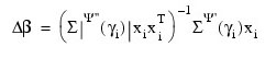
where all derivatives are evaluated at the current estimate of γ and βn+1 = β – ∆β. This step is computed as the estimated regression coefficients in the least-squares model. Step halving is used when necessary to ensure a decrease in the criterion.
- Convergence is assumed when the maximum relative change in any coefficient update from one iteration to the next is less than EPS or when the relative change in the log-likelihood from one iteration to the next is less than EPS/100. Convergence is also assumed after ITMAX iterations or when step halving leads to a step size of less than 0.0001 with no increase in the log-likelihood.
- Residuals are computed according to methods discussed by Pregibon (1981). Let li (γi) denote the log-likelihood of the i-th observation evaluated at γi. Then, the standardized residual is computed as:
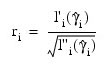
where:

is the value of γi when evaluated at the optimal:

The denominator of this expression is used as the "standard error of the residual" while the numerator is the "raw" residual. Following Cook and Weisberg (1982), the influence of the i-th observation is assumed to be:
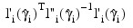
This is a one-step approximation to the change in estimates when the i-th observation is deleted. Here, the partial derivatives are with respect to β.
Programming Notes
- Indicator (dummy) variables are created for the classification variables using IMSL_REGRESSORS with the DUMMY_METHOD keyword set to 1.
- To enhance precision, "centering" of covariates is performed if the model has an intercept and N_observations − N_missing > 1. In doing so, the sample means of the design variables are subtracted from each observation prior to its inclusion in the model. On convergence, the intercept, its variance, and its covariance with the remaining estimates are transformed to the uncentered estimate values.
- Two methods for specifying a binomial distribution model are possible. In the first method, IFREQ contains the frequency of the observation while x(i, irt-1) is 0 or 1 depending upon whether the observation is a success or failure. In this case, x(i, n_Class + n_ Continuous) is always 1. The model is treated as repeated Bernoulli trials, and interval observations are not possible. A second method for specifying binomial models is to use to represent the number of successes in parameter (i) trials. In this case, frequencies will usually be 1.
Example
This example is from Prentice (1976) and involves mortality of beetles after five hours of exposure to eight different concentrations of carbon disulphide. The table below lists the number of beetles exposed (N) to each concentration level of carbon disulphide (x, given as log dosage) and the number of deaths which result (y). The following table shows the data:
|
Log Dosage |
Number of Beetles Exposed
|
Number of Deaths
|
|
1.690 |
59 |
6 |
|
1.724 |
60 |
13 |
|
1.755 |
62 |
18 |
|
1.784 |
56 |
28 |
|
1.811 |
63 |
52 |
|
1.836 |
59 |
53 |
|
1.861 |
62 |
61 |
|
1.883 |
60 |
60 |
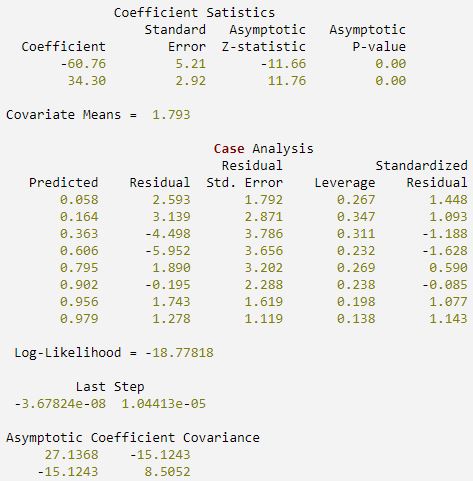
The number of deaths at each concentration level are fitted as a binomial response using the following models: logit (Model = 3), probit (Model = 4), and log-log (Model = 5). Note that the log-log model yields a smaller absolute log likelihood (14.81) than the logit model (18.78) or the probit model (18.23). This is to be expected since the response curve of the log-log model has an asymmetric appearance, but both the logit and probit models are symmetric about θ = 0.5.
.RUN
PRO print_results, cs, means, ca, crit, ls, cov
PRINT, '; Coefficient Statistics'
PRINT, '; Standard Asymptotic ', $
';Asymptotic'
PRINT, '; Coefficient Error Z-statistic ', $
';P-value'
PM, cs, FORMAT = ';(4F13.2)'
PRINT
PRINT, ';Covariate Means = ', means, FORMAT = '(A18, F6.3)'
PRINT
PRINT, '; Case Analysis'
PRINT, '; Residual ', $
';Standardized'
PRINT, '; Predicted Residual Std. Error Leverage', $
'; Residual'
PM, ca, FORMAT = ';(5F12.3)'
PRINT
PRINT, ';Log-Likelihood = ', crit, FORMAT = '(A18, F9.5)'
PRINT
PRINT, '; Last Step'
PRINT, ls
PRINT
PRINT, ';Asymptotic Coefficient Covariance'
PM, cov, FORMAT = ';(2F12.4)'
END
model = 3
nobs = 8
x = ([[1.690, 1.724, 1.755, 1.784, 1.811, 1.836, 1.861, 1.883],$
[6, 13, 18, 28, 52, 53, 61, 60], $
[59, 60, 62, 56, 63, 59, 62, 60]])
ncoef = IMSL_CAT_GLM(0, 1, model, x, Ipar = 2, Eps = 1.0e-3, $
Coef_Stat = cs, Covariances = cov, $
Criterion = crit, Means = means, $
Case_Analysis = ca, Last_Step = ls, Obs_Status = os)
print_results, cs, means, ca, crit, ls, cov
IDL prints:
Errors
Warning Errors
STAT_TOO_MANY_HALVINGS: Too many step halvings. Convergence is assumed.
STAT_TOO_MANY_ITERATIONS: Too many iterations. Convergence is assumed.
Fatal Errors
STAT_TOO_FEW_COEF: INIT_EST is used and N_coef_input = #. The model specified requires # coefficients.
STAT_MAX_CLASS_TOO_SMALL: The number of distinct values of the classification variables exceeds MAX_CLASS = #.
STAT_INVALID_DATA_8: N_CLASS_VALS(#) = #. The number of distinct values for each classification variable must be greater than one.
STAT_NMAX_EXCEEDED: The number of observations to be deleted has exceeded Lp_Max = #. Rerun with a different model or increase the workspace.
Syntax
Result = CAT_GLM(N_class, N_continuous, Model, X [, CASE_ANALYSIS=variable] [, CLASS_VALS=variable] [, COVARIANCES=variable] [, COEF_STAT=variable] [, CRITERION=variable] [, /DOUBLE] [, EPS=value] [, IFIX=value] [, IFREQ=value] [, INDICES_EFFECTS=array] [, INIT_EST=array] [, IPAR=value] [, ITMAX=value] [, LAST_STEP=variable] [, MAX_CLASS=value] [, MEANS=variable] [, N_CLASS_VALS=variable] [, /NO_INTERCEPT] [, OBS_STATUS=variable] [, VAR_EFFECTS=array])
Return Value
An integer value indicating the number of estimated coefficients in the model.
Arguments
Model
The model used to analyze the data. The following table contains the models. The Relationship column refers to the relationship between the parameter, θ or λ, and a linear model of the explanatory variables, Xβ.
|
Model |
Relationship |
PDF of Response Variable
|
|
0 |
Exponential |
Poisson |
|
1 |
Logistic |
Negative Binomial
|
|
2 |
Logistic |
Logarithmic |
|
3 |
Logistic |
Binomial |
|
4 |
Probit |
Binomial |
|
5 |
Log-log |
Binomial |
The lower bound of the response variable is 1 for Model = 3, and it is 0 for all other models. See the description at the beginning of this topic for more information about these models.
N_class
Number of classification variables.
N_continuous
Number of continuous variables.
X
Two-dimensional array of size N_observations by (N_class + N_continuous) + m containing data for the independent variables, dependent variable, and optional parameters.
The columns must be ordered such that the first N_class columns contain data for the class variables, the next N_continuous columns contain data for the continuous variables, and the next column contains the response variable. The final (and optional) m – 1 columns contain optional parameters. See the keywords IFREQ, IFIX, and IPAR.
Keywords
CASE_ANALYSIS (optional)
Named variable containing a two-dimensional array of the case analysis. The array size is [N_observations, 5].
- 0: Predicted mean for the observation if Model = 0. Otherwise, contains the probability of success on a single trial.
- 1: The residual.
- 2: The estimated standard error of the residual.
- 3: The estimated influence of the observation.
- 4: The standardized residual.
Case statistics are computed for all observations except where missing values prevent their computation.
CLASS_VALS (optional)
Named variable into which a one-dimensional array of length:
containing the distinct values of the classification variables in ascending order is stored. The first N_CLASS_VALS(0) elements of CLASS_VALS contain the values for the first classification variables. The next N_CLASS_VALS(1) elements contain the values for the second classification variable, etc.
COVARIANCES (optional)
Named variable into which a two-dimensional array of size [N_coefficients, N_coefficients] containing the estimated asymptotic covariance matrix of the coefficients is stored. For ITMAX = 0, this is the Hessian computed at the initial parameter estimates.
COEF_STAT (optional)
Named variable into which a two-dimensional array of size [N_coefficients, 4] containing the parameter estimates and associated statistics is stored.
- 0: Coefficient Estimate.
- 1: Estimated standard deviation of the estimated coefficient.
- 2: Asymptotic normal score for testing that the coefficient is zero.
- 3: The p-value associated with the normal score in column 2.
CRITERION (optional)
Named variable into which the optimized criterion is stored. The criterion to be maximized is a constant plus the log-likelihood.
DOUBLE (optional)
If present and nonzero, double precision is used.
EPS (optional)
Convergence criterion. Convergence is assumed when the maximum relative change in any coefficient estimate is less than EPS from one iteration to the next or when the relative change in the log-likelihood, criterion, from one iteration to the next is less than EPS/100.0. The default value is 0.001.
IFIX (optional)
Column number Ifix in X containing a fixed parameter for each observation that is added to the linear response prior to computing the model parameter. The fixed parameter allows one to test a hypothesis about the parameters via the log-likelihoods.
IFREQ (optional)
Column number Ifreq in X containing the frequency of response for each observation.
INDICES_EFFECTS (optional)
One-dimensional index array with the following length:
VAR_EFFECTS(0) + VAR_EFFECTS(1) + ... + VAR_EFFECTS(N_effects - 1)
The first VAR_EFFECTS (0) elements give the column numbers of X for each variable in the first effect. The next elements give the column numbers for each variable in the second effect. The last elements give the column numbers for each variable in the last effect. The keywords INDICES_EFFECTS and VAR_EFFECTS must be used together.
INIT_EST (optional)
One-dimensional array of length N_coef_input containing initial estimates of parameters. N_coef_input can be completed by IMSL_REGRESSORS. By default, unweighted linear regression is used to obtain initial estimates.
IPAR (optional)
Column number IPAR in X containing the value of the known distribution parameter for each observation, where X(i, IPAR) is the known distribution parameter associated with the i-th observation. The meaning of the distributional parameter depends upon the model used, as shown in the following table:
|
Model |
Parameter |
Meaning of parameter (i, IPAR) |
| 0 |
E |
ln(E) is a fixed intercept to be included in the linear predictor (i.e., the offset).
|
| 1 |
S |
Number of successes required for the negative binomial distribution |
| 2 |
- |
Not used for this model |
| 3-5 |
N |
Number of trials required for the binomial distribution |
The default behavior is that, when Model ≠ 2, each observation is assumed to have a parameter value of 1. When Model = 2, this parameter is not referenced.
ITMAX (optional)
Maximum number of iterations. Use a value of 0 to compute Hessian (stored in COVARIANCES), and the Newton step (stored in LAST_STEP) at the initial estimates. Use the keyword INIT_EST to get the initial estimates. The default value is 30.
LAST_STEP (optional)
Named variable in the form of a one-dimensional array of length N_coefficients containing the last parameter updates (excluding step halvings). When ITMAX is set to 0, LAST_STEP contains the inverse of the Hessian times the gradient vector, all computed at the initial parameter estimates.
MAX_CLASS (optional)
An upper bound on the sum of the number of distinct values taken on by each classification variable. The default value is N_observations by N_class.
MEANS (optional)
Named variable in the form of a one-dimensional array containing the means of the design variables. The array is of length N_coefficients if the keyword NO_INTERCEPT is used, and N_Coefficients − 1 otherwise.
N_CLASS_VALS (optional)
Named variable in the form of a one-dimensional array of length N_class containing the number of values taken by each classification variable. The i-th classification variable has N_CLASS_VALS (i) distinct values.
NO_INTERCEPT (optional)
If present and nonzero, there is no intercept in the model. By default, the intercept is automatically included in the model.
OBS_STATUS (optional)
Named variable into which an one-dimensional array of length N_observations indicating which observations are included in the extended likelihood is stored.
- 0: Observation i is in the likelihood
- 1: Observation i cannot be in the likelihood because it contains at least one missing value in X.
- 2: Observation i is not in the likelihood. Its estimated parameter is infinite.
Notes
- Dummy variables are generated for the classification variables as follows: An ascending list of all distinct values of each classification variable is obtained and stored in CLASS_VALS. Dummy variables are then generated for each but the last of these distinct values. Each dummy variable is zero unless the classification variable equals the list value corresponding to the dummy variable, in which case the dummy variable is one. See the input keyword DUMMY_METHOD = 1 in IMSL_REGRESSORS.
- The "product" of a classification variable with a covariate will yield dummy variables equal to the product of the covariate, with each of the dummy variables associated with the classification variable.
- The "product" of two classification variables will yield dummy variables in the usual manner. Each dummy variable associated with the first classification variable multiplies each dummy variable associated with the second classification variable. The resulting dummy variables are such that the index of the second classification variable varies fastest.
VAR_EFFECTS (optional)
One-dimensional array of length N_effects containing the number of variables associated with each effect in the model, where N_effects is the number of effects (source of variation) in the model. Keywords VAR_EFFECTS and INDICES_EFFECTS must be used together.
Version History