The IMSL_GENEIG procedure computes the generalized eigenexpansion of a system Ax = λBx.
This routine requires an IDL Advanced Math and Stats license. For more information, contact your sales or technical support representative.
The IMSL_GENEIG function uses the QZ algorithm to compute the eigenvalues and eigenvectors of the generalized eigensystem Ax = λBx, where A and B are matrices of order n. The eigenvalues for this problem can be infinite, so α and β are returned instead of λ. If β is nonzero, λ = α/β.
The QZ algorithm first simultaneously reduces A to upper-Hessenberg form and B to upper-triangular form, then it uses orthogonal transformations to reduce A to quasiupper- triangular form while keeping B upper triangular. The generalized eigenvalues and eigenvectors for the reduced problem are then computed.
The IMSL_GENEIG function is based on the QZ algorithm due to Moler and Stewart (1973), as implemented by the EISPACK routines QZHES, QZIT, and QZVAL; see Garbow et al. (1977).
Examples
Example 1
This example computes the eigenvalue, λ, of system Ax = λBx, where:
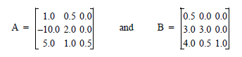
a = TRANSPOSE([[1.0, 0.5, 0.0], [-10.0, 2.0, 0.0], $
[5.0, 1.0, 0.5]])
b = TRANSPOSE([[0.5, 0.0, 0.0], [3.0, 3.0, 0.0], $
[4.0, 0.5, 1.0]])
IMSL_GENEIG, a, b, alpha, beta
PM, alpha/beta, Title = 'Eigenvalues'
IDL prints:
Eigenvalues
( 0.833334, 1.99304)
( 0.833333, -1.99304)
( 0.500000, 0.00000)
Example 2
This example finds the eigenvalues and eigenvectors of the same eigensystem given in the last example.
a = TRANSPOSE([[1.0, 0.5, 0.0], [-10.0, 2.0, 0.0], $
[5.0, 1.0, 0.5]])
b = TRANSPOSE([[0.5, 0.0, 0.0], [3.0, 3.0, 0.0], $
[4.0, 0.5, 1.0]])
IMSL_GENEIG, a, b, alpha, beta, Vectors = vectors
PM, alpha/beta, Title = 'Eigenvalues'
IDL prints:
Eigenvalues
( 0.833332, 1.99304)
( 0.833332, -1.99304)
( 0.500000, -0.00000)
Continue:
PM, vectors, Title = 'Eigenvectors'
IDL prints:
Eigenvectors
( -0.197112, 0.149911)( -0.197112, -0.149911)( -1.53306e-08, 0.00000)
( -0.0688163, -0.567750)( -0.0688163, 0.567750)( -4.75248e-07, 0.00000)
( 0.782047, 0.00000)( 0.782047, 0.00000)( 1.00000, 0.00000)
Example 3
This example solves the eigenvalue, λ, of system Ax = λBx, where:
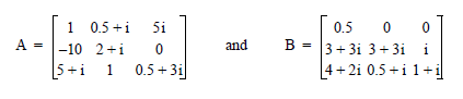
a = TRANSPOSE([$
[COMPLEX(1.0, 0.0), COMPLEX(0.5, 1.0), COMPLEX(0.0, 5.0)], $
[COMPLEX(-10.0, 0.0), COMPLEX(2.0, 1.0), COMPLEX(0.0, 0.0)], $
[ COMPLEX(5.0, 1.0), COMPLEX(1.0, 0.0), COMPLEX(0.5, 3.0)]])
b = TRANSPOSE([$
[COMPLEX(0.5, 0.0), COMPLEX(0.0, 0.0), COMPLEX(0.0, 0.0)], $
[COMPLEX(3.0, 3.0), COMPLEX(3.0, 3.0), COMPLEX(0.0, 1.0)], $
[COMPLEX(4.0, 2.0), COMPLEX(0.5, 1.0), COMPLEX(1.0, 1.0)]])
IMSL_GENEIG, a, b, alpha, beta
PM, alpha/beta, Title = 'Eigenvalues'
IDL prints:
Eigenvalues
( -8.18016, -25.3799)
( 2.18006, 0.609113)
( 0.120108, -0.389223)
Example 4
This example finds the eigenvalues and eigenvectors of the same eigensystem given in the last example.
a = TRANSPOSE([$
[COMPLEX(1.0, 0.0), COMPLEX(0.5, 1.0), COMPLEX(0.0, 5.0)], $
[COMPLEX(-10.0, 0.0), COMPLEX(2.0, 1.0), COMPLEX(0.0, 0.0)], $
[COMPLEX(5.0, 1.0), COMPLEX(1.0, 0.0), COMPLEX(0.5, 3.0)]])
b = TRANSPOSE([$
[COMPLEX(0.5, 0.0), COMPLEX(0.0,0.0), COMPLEX(0.0, 0.0)], $
[COMPLEX(3.0,3.0), COMPLEX(3.0,3.0), COMPLEX(0.0, 1.0)], $
[COMPLEX(4.0, 2.0), COMPLEX(0.5, 1.0), COMPLEX(1.0, 1.0)]])
IMSL_GENEIG, a, b, alpha, beta, Vectors = vectors
PM, alpha/beta, Title = 'Eigenvalues'
IDL prints:
Eigenvalues
( -8.18018, -25.3799)
( 2.18006, 0.609112)
( 0.120109, -0.389223)
Continue:
PM, vectors, Title = 'Eigenvectors'
IDL prints:
Eigenvectors
( -0.326709, -0.124509)( -0.300678, -0.244401)( 0.0370698, 0.151778)
( 0.176670, 0.00537758)( 0.895923, 0.00000)( 0.957678, 0.00000)
( 0.920064, 0.00000)( -0.201900, 0.0801192)( -0.221511, 0.0968290)
Syntax
IMSL_GENEIG, A, B, Alpha, Beta [, /DOUBLE] [, VECTORS=variable]
Arguments
A
Two-dimensional array of size n-by-n containing coefficient matrix A.
Alpha
One-dimensional array of size n containing scalars αi. If βi ≠ 0, λi = αi /βi for i = 0, ..., n – 1 are the eigenvalues of the system.
B
Two-dimensional array of size n-by-n containing coefficient matrix B.
Beta
One-dimensional array of size n.
Keywords
DOUBLE (optional)
If present and nonzero, double precision is used.
VECTORS (optional)
Named variable into which a two-dimensional array of size n-by-n containing eigenvectors of the problem is stored. Each vector is normalized to have Euclidean length equal to one.
Version History