The IMSL_LINPROG function solves a linear programming problem using the revised simplex algorithm.
This routine requires an IDL Advanced Math and Stats license. For more information, contact your sales or technical support representative.
The IMSL_LINPROG function uses a revised simplex method to solve linear programming problems; i.e., problems of the form:

subject to:
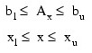
where c is the objective coefficient vector, A is the coefficient matrix, and the vectors bl, bu, xl, and xu are the lower and upper bounds on the constraints and the variables. For a complete discussion of the revised simplex method, see Murtagh (1981) or Murty (1983). This problem can be solved more efficiently.
Example
In this example, the linear programming problem in the standard form:
In this example, the linear programming problem in the standard form:
min f(x) = –x0 – 3x1
subject to:
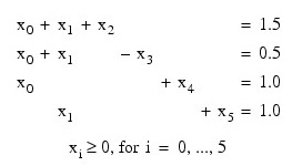
is solved.
a = [[1, 1, 1, 0],$
[1, 1, 0, 1],$
[1, 0, 0, 0],$
[0, (-1), 0, 0],$
[0, 0, 1, 0],$
[0, 0, 0, 1]]
b = [1.5,.5,1,1]
c = [(-1),(-3),0,0,0,0]
PM, IMSL_LINPROG(a, b, c), Title = ';Solution'
IDL prints:
Solution
0.500000
1.00000
0.00000
1.00000
0.500000
0.00000
Errors
Warning Errors
MATH_PROB_UNBOUNDED: Problem is unbounded.
MATH_TOO_MANY_ITN: Maximum number of iterations exceeded.
MATH_PROB_INFEASIBLE: Problem is infeasible.
Fatal Errors
MATH_NUMERIC_DIFFICULTY: Numerical difficulty occurred. If float is currently being used, using double may help.
MATH_BOUNDS_INCONSISTENT: Bounds are inconsistent.
Syntax
Result = IMSL_LINPROG(A, B, C [, BU=array] [, /DOUBLE] [, DUAL=variable] [, IRTYPE=array] [, ITMAX=value] [, OBJ=variable] [, XLB=array] [, XUB=array])
Return Value
The solution x of the linear programming problem.
Arguments
A
Two-dimensional matrix containing the coefficients of the constraints. The coefficient for the i-th constraint is contained in A (i, *).
B
One-dimensional matrix containing the right-hand side of the constraints. If there are limits on both sides of the constraints, b contains the lower limit of the constraints.
C
One-dimensional array containing the coefficients of the objective function.
Keywords
BU
Array with N_ELEMENTS(b) elements containing the upper limit of the constraints that have both the lower and the upper bounds. If no such constraint exists, BU is not needed.
DOUBLE (optional)
If present and nonzero, then double precision is used.
DUAL (optional)
Name of the variable into which the array with N_ELEMENTS(c) elements, containing the dual solution, is stored.
IRTYPE (optional)
Array with N_ELEMENTS(b) elements indicating the types of general constraints in the matrix A. Let ri = Ai0x0 + ... + Ain–1 xn–1. The value of IRTYPE (i) is described below. The default is IRTYPE (*) = 0.
|
IRTYPE (i) |
Constraints |
|
0 |
ri = bi
|
|
1 |
ri ≤ bu
|
|
2 |
ri ≥ bi
|
|
3 |
bi ≤ ri ≤ bu
|
ITMAX (optional)
Maximum number of iterations. Default: 10,000
OBJ (optional)
Name of the variable into which the optimal value of the objective function is stored.
XLB (optional)
Array with N_ELEMENTS(c) elements containing the lower bound on the variables. If there is no lower bound on a variable, 1030 should be set as the lower bound. Default: (*) = 0
XUB (optional)
Array with N_ELEMENTS(c) elements containing the upper bound on the variables. If there is no upper bound on a variable, –1030 should be set as the upper bound. Default: (*) = infinity
Version History