The IMSL_ODE function solves an initial value problem, which is possibly stiff, using the Adams-Gear methods for ordinary differential equations. Using keywords, the Runge-Kutta-Verner fifth-order and sixth-order method can be used if you know the problem is not stiff.
This routine requires an IDL Advanced Math and Stats license. For more information, contact your sales or technical support representative.
The IMSL_ODE function finds an approximation to the solution of a system of first- order differential equations of the form:
with given initial conditions for y at the starting value for t. The function attempts to keep the global error proportional to a user-specified tolerance. The proportionality depends on the differential equation and the range of integration.
The function returns a two-dimensional array with the (i, j)-th component containing the i-th approximate solution at the j-th time step. Thus, the returned matrix has dimension (N_ELEMENTS (y), N_ELEMENTS (t)). It is important to notice here that the initial values of the problem also are included in this two-dimensional matrix.
The code is based on using backward differentiation formulas not exceeding order five as outlined in Gear (1971) and implemented by Hindmarsh (1974). There is an optional use of the code that employs implicit Adams formulas. This use is intended for nonstiff problems with expensive functions y′ = f(t, y).
If the keyword R_K_V is set, the IMSL_ODE function uses the Runge-Kutta-Verner fifth-order and sixth-order method and is efficient for nonstiff systems where the evaluations of f(t, y) are not expensive. The code is based on an algorithm designed by Hull et al. (1976) and Jackson et al. (1978) and uses Runge-Kutta formulas of order five and six developed by J.H. Verner.
Examples
Example 1
This is a mildly stiff example problem (F2) from the test set of Enright and Pryce (1987).
.RUN
y'1 = –k1y1 + k2 (1 – y1) y0
y'1 = –k1y1 + k2 (1 – y1) y0
y0(0) = 1
y1(0) = 0
k0 = 294
k1 = 3
k2 = 0.01020408
.RUN
FUNCTION f, t, y
RETURN, [-y(0) - y(0) * y(1) + 294. * y(1), $
-3.*y(1) + 0.01020408*(1. - y(1)) * y(0)]
END
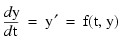
yp = IMSL_ODE([0, 120, 240], [1, 0], 'f')
PM, yp, FORMAT = '(3f10.6)', $
Title = ' y(0) y(120) y(240)'
IDL prints:
Now solve the same problem but with a user supplied Jacobian.
.RUN
FUNCTION f, t, y
RETURN, [-y(0)-y(0)*y(1)+294.0*y(1), $
-3.0*y(1)+0.01020408*(1.0-y(1))*y(0)]
END
.RUN
FUNCTION jacob, x, y, dydx
dydx = [ [-y(1)-1,0.01020408*(1-y(1))], $
[294-y(0),-0.01020408*y(0)-3] ]
RETURN, dydx
END
yp = IMSL_ODE( [0,120,240], [1,0], 'f', JACOBIAN='jacob', MITER=2)
PM, yp, FORMAT='(3f10.6)', TITLE=' y(0) y(120) y(240)'
Example 2
Runge-Kutta Method
This example solves:

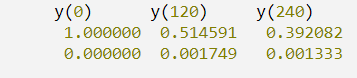
over the interval [0, 1] with the initial condition y(0) = 1 using the Runge-Kutta- Verner fifth-order and sixth-order method. The solution is y(t) = e–t.
.RUN
FUNCTION f, t, y
RETURN, -y
END
yp = IMSL_ODE([0, 1], [1], 'f', /R_K_V)
PM, yp, Title = 'Solution'
IDL prints:
Example 3
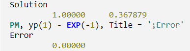
Predator-Prey Problem
Consider a predator-prey problem with rabbits and foxes. Let r be the density of rabbits, and let f be the density of foxes. In the absence of any predator-prey interaction, the rabbits would increase at a rate proportional to their number, and the foxes would die of starvation at a rate proportional to their number. Mathematically, the model without species interaction is approximated by the following equations:

With species interaction, the rate at which the rabbits are consumed by the foxes is assumed to equal the value 2rf. The rate at which the foxes increase because they are consuming the rabbits, is equal to rf. Thus, the model differential equations to be solved are as follows:

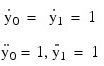
For illustration, the initial conditions are taken to be r(0) = 1 and f(0) = 3. The interval of integration is 0 ≤ t ≤ 40. In the program, y(0) = r and y(1) = f. The IMSL_ODE function is then called with 100 time values from 0 to 40. The results are shown in the figure that follows.
.RUN
FUNCTION f, t, y
yp = y
yp(0) = 2 * y(0) * (1 - y(1))
yp(1) = -y(1) * (1 - y(0))
RETURN, yp
END
y = [1, 3]
t = 40 * FINDGEN(100)/99
y = IMSL_ODE(t, y, 'f', /R_K_V)
PLOT, y(0, *), y(1, *), Psym = 2, XTitle = 'Density of Rabbits', $
YTitle = 'Density of Foxes'
Example 4
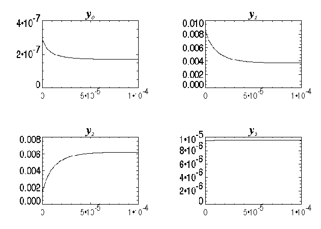
Stiff Problems and Changing Defaults
This problem is a stiff example (F5) from the test set of Enright and Pryce (1987). An initial step size of h = 10–7 is suggested by these authors. When solving a problem that is known to be stiff, using double precision is advisable. The IMSL_ODE function is forced to use the suggested initial step size and double precision by using keywords.
y'0 = k0( –k1y0y1 + k2y3 – k3 y0y2)
y'1 = k0k1y0y1 + k4y3
y'2 = k0 ( –k3y0y2 + k5y3)
y'3 = k0 ( k1y0y1 – k2y3 + k3 y0y2 )
y0(0) = 3.365 x 10⁻⁷
y1(0) = 8.261 x 10⁻³
y2(0) = 1.641 x 10⁻³
y3(0) = 9.380 x 10⁻⁶
k0 = 1011
k1 = 3
k2 = 0.0012
k3 = 9
k4 = 2 x 10⁷
k5 = 0.001
The results are shown in the figure that follows.
.RUN
FUNCTION f, t, y
k = [1d11, 3., .0012, 9., 2d7, .001]
yp = [k(0)*(-k(1)*y(0)*y(1)+k(2)*y(3)- $
k(3)*y(0)*y(2)),-k(0)*k(1)*y(0)*y(1)+ $
k(4)*y(3),k(0)*(-k(3)*y(0)*y(2) + $
k(5)*y(3)),k(0)* (k(1)*y(0)*y(1)- $
k(2)*y(3)+k(3)*y(0)*y(2))]
RETURN, yp
END
t = FINDGEN(500)/5e6
y = [3.365e-7, 8.261e-3, 1.641e-3, 9.380e-6]
y = IMSL_ODE(t, y, 'f', Hinit = 1d-7, /Double)
!P.Multi = [0, 2, 2]
!P.Font = 0
PLOT, t, y(0, *), Title = '!8y!I0!5', XTICKS=2
PLOT, t, y(1, *), Title = '!8y!I1!5', XTICKS=2
PLOT, t, y(2, *), Title = '!8y!I2!5', XTICKS=2
PLOT, t, y(3, *), Title = '!8y!I3!5', XTICKS=2
Example 5
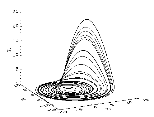
Strange Attractors, the Rossler System
This example illustrates a strange attractor. The strange attractor used is the Rossler system, a simple model of a truncated Navier-Stokes equation. The Rossler system is given by relation below.
y'0 = – y1 – y2
y'1 = y0 + a y1
y'2 = b + y0 y2 – c y2
The initial conditions and constants are shown below.
y0(0) = 1
y1(0) = 0
y2(0) = 0
a = 0.2
b = 0.2
c = 5.7
.RUN
FUNCTION f, t, y
COMMON constants, a, b, c
yp(0) = -y(1) - y(2)
yp(1) = y(0) + a * y(1)
yp(2) = b + y(0) * y(2) - c * y(2) RETURN, yp
END
COMMON constants, a, b, c a = .2
b = .2
c = 5.7
t = FINDGEN(ntime)/(ntime - 1) * time_range y = [1, 0, 0]
y = IMSL_ODE(t, y, 'f', Max_Steps = max_steps, /Double)
!P.Charsize = 1.5
SURFACE, FINDGEN(2, 2), /Nodata, $
XRange = [MIN(y(0, *)), MAX(y(0, *))], $
YRange = [MIN(y(1, *)), MAX(y(1, *))], $
ZRange = [MIN(y(2, *)), MAX(y(2, *))], $
XTitle = '!6y!i0', YTitle = 'y!i1', $
ZTitle = 'y!i2', Az = 25, /Save
PLOTS, y(0, *), y(1, *), y(2, *), /T3d
Example 6
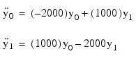
Coupled, Second-order System
Consider the two-degrees-of-freedom system represented by the model (and corresponding free-body diagrams) in the figure that follows. Assuming y1 is greater than y0 causes the spring k1 to be in tension, as seen by the tensile force k1 (y1 – y0).
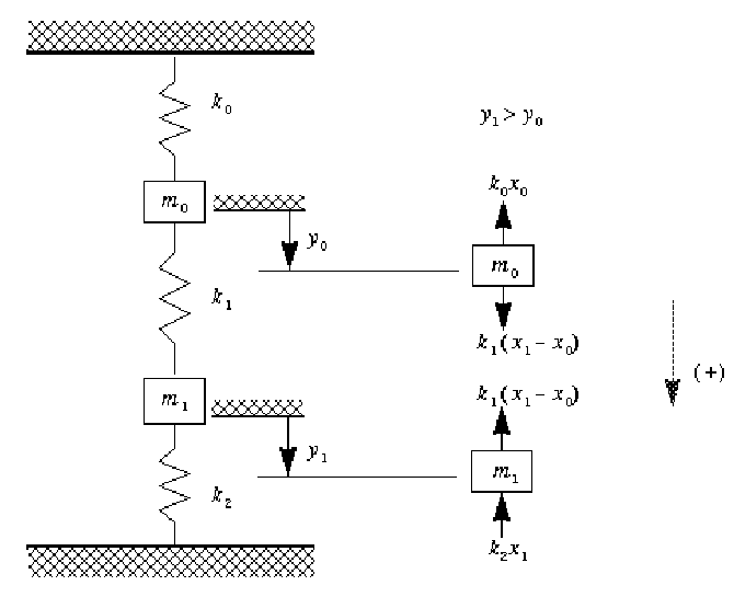
Note: If y0 is taken to be greater than y1, then spring k1 is in compression, with the spring force k1 (y0 – y1). Both methods give correct results when a summation of forces is written.
The differential equations of motion for the system are written as follows:
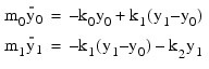
Thus:
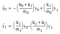
If given the mass and spring constant values:
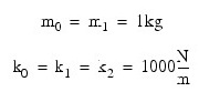
the following is true:
Now, in order to convert this problem into one which IMSL_ODE can be used to solve, choose the following variables:
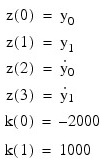
which yields the following equations:
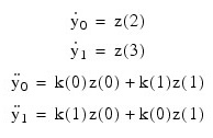
The last four equations are the object of the return values of the user-supplied function in the exact order as previously specified.
The example below loops through four different sets of initial values for z. The results are shown below.
.RUN
FUNCTION f, t, z
k = [-2000, 1000]
RETURN, [z(2), z(3), k(0) * z(0) + k(1) * $
z(1), k(1) * z(0) + k(0) * z(1)]
END
.RUN
t = FINDGEN(1000)/999
!P.MULTI = [0, 2, 2]
FOR i = 0, 3 DO BEGIN
z = [1, i/3., 0, 0]
z = IMSL_ODE(t, z, 'f', Max_Steps = 1000, Hinit = 0.001, /R_K_V)
PLOT, t, z(0, *), Thick = 2, Title = 'Displacement of Mass'
OPLOT, t, z(1, *), Linestyle = 1, Thick = 2
ENDFOR
END
The displacement for m0 is the solid line, and the dotted line represents the displacement for m1. Note that when the initial conditions for:
 and
and 
are equal, the displacement of the masses is equal for all values of the independent variable (as seen in the fourth plot). Also, the two principal modes of this problem occur when the following is true:
Errors
Fatal Errors
MATH_ODE_TOO_MANY_EVALS: Completion of the next step would make the number of function evaluations #, but only # evaluations are allowed.
MATH_ODE_TOO_MANY_STEPS: Maximum number of steps allowed; # used. The problem may be stiff.
MATH_ODE_FAIL: Unable to satisfy the error requirement. TOLERANCE = # may be too small.
Syntax
Result = IMSL_ODE(T, Y, F [, /DOUBLE] [, FLOOR=value] [, HINIT=value] [, HMAX=value] [, HMIN=value] [, MAX_EVALS=value] [, MAX_STEPS=value] [, N_STEPS=variable] [, N_EVALS=variable] [, NORM=value] [, R_K_V=value] [, SCALE=value] [, TOLERANCE=value] [, JACOBIAN=string] [, MAX_ORD=value] [, METHOD=value] [, MITER=value] [, N_JEVALS=value])
Return Value
A two-dimensional array containing the approximate solutions for each specified value of the independent variable. The elements (i, *) are the solutions for the i-th variable.
Arguments
T
One-dimensional array containing values of the independent variable. Parameter t(0) should contain the initial independent variable value, and the remaining elements of t should be filled with values of the independent variable at which a solution is desired.
Y
Array containing the initial values of the dependent variables.
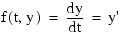
F
Scalar string specifying a user-supplied function to evaluate the right-hand side. This function takes two parameters, t and y, where t is the current value of the independent variable and y is defined above.
The return value of this function is an array defined by the following equation:
Keywords
DOUBLE (optional)
If present and nonzero, then double precision is used.
FLOOR (optional)
Used with IMSL_NORM. Provides a positive lower bound for the error norm option with value 2. Default: 1.0
HINIT (optional)
Scalar value used for the initial value for the step size h. Steps are applied in the direction of integration. Default: 0.001 | t (i + 1 ) – t (i) |
HMAX (optional)
Scalar value used as the maximum value for the step size h. If keyword R_K_V is set, HMAX = 2.0 is used. Default: largest machine-representable number.
HMIN (optional)
Scalar value used as the minimum value for the step size h. Default: 0.0
MAX_EVALS (optional)
Integer value used in the maximum number of function evaluations allowed per time step. Default: no enforced limit.
MAX_STEPS (optional)
Integer value used in the maximum number of steps allowed per time step. Default: 500.
N_STEPS (optional)
Named variable into which the array containing the number of steps taken at each value of t is stored.
N_EVALS (optional)
Named variable into which the array containing the number of function evaluations used at each value of t is stored.
NORM (optional)
Switch determining the error norm. The default is 0. In the following, ei is the absolute value of the error estimate for yi.
- 0: Minimum of the absolute error and the relative error equals the maximum of ei/max ( |yi|, 1) for i = 0, ..., N_ELEMENTS (y) – 1.
- 1: Absolute error, equals maxiei.
- 2: The error norm is maxi(ei/wi), where wi = max ( |yi|, Floor).
R_K_V (optional)
If present and nonzero, uses the Runge-Kutta-Verner fifth-order and sixth-order method.
SCALE (optional)
Scalar value used as a measure of the scale of the problem, such as an approximation to the Jacobian along the trajectory. Default: 1
TOLERANCE (optional)
Scalar value used to set the tolerance for error control. An attempt is made to control the norm of the local error such that the global error is proportional to TOLERANCE. Default: 0.001
The following keywords are for the Adams Gear (Default) method only:
JACOBIAN (optional)
Scalar string specifying a user-supplied function to evaluate the Jacobian matrix. This function takes three parameters, x, y, and yprime, where x and y are defined in the description of the argument F and yprime is the array returned by the user-supplied argument F. The return value of this function is a two-dimensional array containing the partial derivatives. Each derivative ∂y'i / ∂yj is evaluated at the provided (x, y) values and is returned in array location (i, j).
MAX_ORD (optional)
Defines the highest order formula of implicit Adams type or BDF type to use. Default: value 12 for Adams formulas; value 5 for BDF formulas
METHOD (optional)
Chooses the class of integration methods. The default is 2:
- 1: Uses implicit Adams method.
- 2: Uses backward differentiation formula (BDF) methods.
MITER (optional)
Chooses the method for solving the formula equations. The default is 3:
- 1: Uses function iteration or successive substitution.
- 2: Uses chord or modified Newton method and a user-supplied Jacobian matrix.
- 3: Same as 2 except Jacobian is approximated within the function by divided differences.
N_JEVALS (optional)
Named variable into which the array containing the number of Jacobian function evaluations used at each value of t is stored. The values returned are nonzero only if the keyword JACOBIAN is also used.
Version History
See Also
IMSL_NORM