The IMSL_ARMA function computes method-of-moments or least-squares estimates of parameters for a nonseasonal IMSL_ARMA model.
This routine requires an IDL Advanced Math and Stats license. For more information, contact your sales or technical support representative.
The IMSL_ARMA function computes estimates of parameters for a nonseasonal IMSL_ARMA model given a sample of observations, {Zt}, for t = 1, 2, ..., n, where n = N_ELEMENTS(Z). You may choose either method of moments or least squares. The default is method of moments.
Choose the method-of-moments algorithm with the keyword MOMENTS. The least-squares algorithm is used if LSQ is specified. If you wish to use the least-squares algorithm, the preliminary estimates are the method-of-moments estimates by default; otherwise, you can input initial estimates by specifying keywords INIT_EST_AR and INIT_EST_MA. The table below lists the appropriate keywords for both the method-of-moments and least-squares algorithm:
|
Method of Moments only
|
Least Squares only
|
Both Method of Moments and Least Squares
|
|
MOMENTS |
LSQ |
ERR_REL |
|
|
CONSTANT (or NO_CONSTANT)
|
ITMAX |
|
|
AR_LAGS |
MEAN_ESTIMATE |
|
|
MA_LAGS |
AUTOCOV |
|
|
LGTH_BACKCAST |
FORECAST |
|
|
TOL_BACKCAST |
N_PREDICT |
|
|
INIT_EST_AR |
CONFIDENCE |
|
|
RESIDUAL |
BACKWARD_ORIGIN |
|
|
INIT_EST_MA |
|
|
|
PARAM_EST_COV |
|
|
|
SS_RESIDUAL |
|
Method-of-moments Estimation
Suppose the time series {Zt} is generated by an IMSL_ARMA(p, q) model of the form:
φ(B )Zt = θ0 + θ(B )At
for
t ∈ {0, ±1, ±2, ... }
let
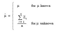
µˆ = Mean_Est
be the estimate of the mean µ of the time series {Zt}, where:
µˆ
equals the following:
The autocovariance function is estimated by:
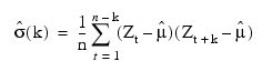
for k = 0, 1, ..., K, where K = p + q + 1. Note that:

is an estimate of the sample variance.
Given the sample autocovariances, the function computes the method-of-moments estimates of the autoregressive parameters using the extended Yule-Walker equations as follows:

where:
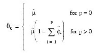
The overall constant θ0 is estimated by the following:
The moving average parameters are estimated based on a system of nonlinear equations given K = p + q + 1 autocovariances, σ(k) for k = 1, ..., K, and p autoregressive parameters φi for i = 1, ..., p.
Let Z't = φ(B)Zt. The autocovariances of the derived moving average process Z't = θ(B)At are estimated by the following relation:
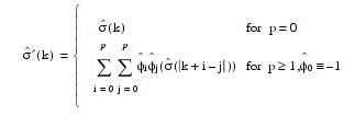
The iterative procedure for determining the moving average parameters is based on the relation:
where σ(k) denotes the autocovariance function of the original Zt process.
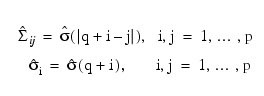
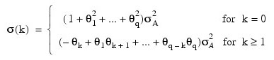
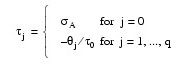
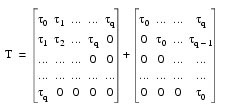
Let τ = (τ0, τ1, ..., τq)T, f = (f0, f1, ..., fq)T, and T be a (q + 1) x (q + 1) matrix, where τj, fj , and T are as follows:
and:
Then, the value of τ at the (i + 1)-th iteration is determined by:
τ i + 1 = τ i – (T i)–1 f i
The estimation procedure begins with the initial value:
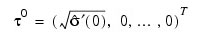
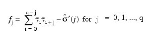
and terminates at iteration i when either |f i| is less than Err_Rel or i equals Itmax. The moving average parameter estimates are obtained from the final estimate of τ by setting:

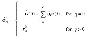
for j = 1, ..., q. The random error variance is estimated by the following:
See Box and Jenkins (1976, pp. 498–500) for a description of a function that performs similar computations.
Least-squares Estimation
Suppose the time series {Zt} is generated by a nonseasonal IMSL_ARMA model of the form:
φ(B )(Zt – µ ) = θ(B)At , for t ∈ {0, ±1, ±2, …}
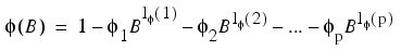
where B is the backward-shift operator, µ is the mean of Zt , and:
with p autoregressive and q moving average parameters. Without loss of generality, the following is assumed:
so that the nonseasonal IMSL_ARMA model is of order (p', q'), where:
p′ = lφ(p ) and q′ = lθ(q)
Note that the usual hierarchical model assumes the following:
Consider the sum-of-squares function:
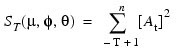
where:
and T = Lgth_Backcast is the length of backcasting from the beginning of the series. The random errors {At } are assumed to be independent and identical distributed N(0, σA2) random variables. Hence, the log-likelihood function is given by:
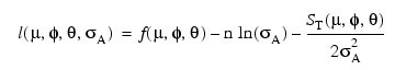
where f (µ, φ, θ) is a function of µ, φ, and θ.
For T = 0, the log-likelihood function is conditional on the past values of both Zt and At required to initialize the model. The method of selecting these initial values usually introduces transient bias into the model (Box and Jenkins 1976, pp. 210–211). For T = infinity, this dependency vanishes, and the estimation problem concerns maximization of the unconditional log-likelihood function. Box and Jenkins (1976, p. 213) argue that:
S (µ, φ, θ) (⁄ 2σ2 )
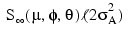 dominates
The parameter estimates that minimize the sum-of-squares function are called least- squares estimates. For large n, the unconditional least-squares estimates are approximately equal to the maximum likelihood-estimates.
In practice, a finite value of T enables sufficient approximation of the unconditional sum-of-squares function. The values of [At] needed to compute the unconditional sum of squares are computed iteratively with initial values of Zt obtained by backcasting. The residuals (including backcasts), estimate of random error variance, and covariance matrix of the final parameter estimates also are computed. ARIMA parameters can be computed using the IMSL_DIFFERENCE, together with IMSL_ARMA.
Forecasting Option
The Box-Jenkins forecasts and their associated confidence intervals for a nonseasonal IMSL_ARMA model are computed given a sample of n = N_ELEMENTS(z) {Zt} for t = 1, 2, ..., n.
Suppose the time series {Zt} is generated by a nonseasonal IMSL_ARMA model of the form:
φ (B) Zt = θ0 + θ (B) At
for t ∈ { 0, ±1, ±2, … }
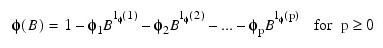
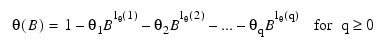
where B is the backward-shift operator, θ0 is the constant, and:
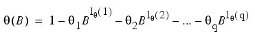
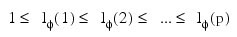
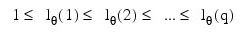
with p autoregressive and q moving average parameters. Without loss of generality, the following is assumed:
so that the nonseasonal IMSL_ARMA model is of order (p', q'), where:
 and
and 
Note that the usual hierarchal model assumes the following:
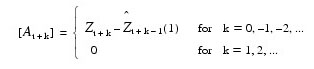
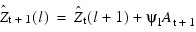
The Box-Jenkins forecast at origin t for lead time l of Zt + l is defined in terms of the difference equation:
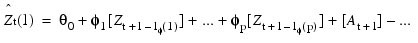
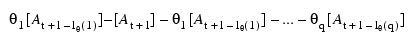
where the following is true:
The 100(1 – α)-percent confidence interval for Zt + l is given by:
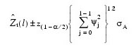
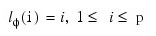
where z(1 – α ⁄ 2 ) is the 100 (1 – α / 2)-percentile of the standard normal distribution, σA is the standard deviation of the random error, and ψj is defined as follows:
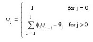
In this equation, φi = 0 for i > p and θj = 0 for j > q. Note that the forecasts are computed for lead times l = 1, 2, ..., L at origins t = (n – b), (n – b + 1), ..., n, where L = N_Predict and b = Backward_Origin.
The Box-Jenkins forecasts minimize the mean-square error:
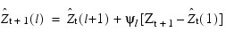
Also, the forecasts are easily updated according to the following equation:
This approach and others are discussed in Chapter 5 of Box and Jenkins (1976).
Examples
Example 1
Consider the Wolfer Sunspot Data (Anderson 1971, p. 660) consisting of the number of sunspots observed each year from 1749 through 1924. The data set for this example consists of the number of sunspots observed from 1770 through 1869 and is shown in the figure that follows. The method-of-moments estimates:
 and
and 
for the IMSL_ARMA(2,1) model are:

where Zt is “raw” data and the errors At are independently and identical normally distributed with mean zero and variance σ2A.
temp = IMSL_STATDATA(2)
PLOT, years, z, XStyle = 1, Psym = -6, $
Title = 'Wolfer Sunspot Data', XTitle = 'Year', $
YTitle = 'Number of Sunspots'
q = 1
parameters = IMSL_ARMA(z, p, q)
PRINT, 'AR estimates:', parameters(1), parameters(2) PRINT, 'MA estimate :', parameters(3)
IDL prints:
AR estimates: 1.24426 -0.575149
MA estimate : -0.124094
The following is the Wolfer Sunspot Data Plot:
Example 2
The data for this example are the same as that for the initial example. Preliminary method-of-moments estimates are computed by default, and the method of least squares is used to find the final estimates.
temp = IMSL_STATDATA(2)
z = TEMP(21:120, 1)
parameters = IMSL_ARMA(z, 2, 1, /Lsq)
PRINT, 'AR estimates:', parameters(1), parameters(2) PRINT, 'MA estimate :', parameters(3)
AR estimates: 1.39257 -0.732948
MA estimate : -0.137512
Example 3
Consider the Wolfer Sunspot Data (Anderson 1971, p. 660) consisting of the number of sunspots observed each year from 1749 through 1924. The data set for this example consists of the number of sunspots observed from 1770 through 1869. IMSL_ARMA computes forecasts and 95-percent confidence limits for the forecasts for an IMSL_ARMA(2, 1) model fit using IMSL_ARMA with the
method-of-moments option. With Backward_Origin = 3, columns zero through three
of Forecast provide forecasts given the data through 1866, 1867, 1868, and 1869. Column five gives the deviations from the forecast for computing confidence limits, and column six gives the psi weights, which can be used to update forecasts when more data is available. For example, the forecast for the 102-nd observation (year
1871) given the data through the 100-th observation (year 1869) is 77.21; 95-percent confidence limits are given by:

After observation 101 (Z101 for year 1870) is available, the forecast can be updated by using:
with the psi weight (ψ1 = 1.37) and the one-step-ahead forecast error for observation 101 (Z101 – 83.72) to give the following:
77.21 + 1.37 x (Z101 – 83.72)
Since this updated forecast is one step ahead, the 95-percent confidence limits are now given by the forecast:

First, define a procedure to output the results:
.RUN
PRO print_results, parameters, forecast
PRINT, 'Method-of-moments initial estimates:'
PRINT, 'AR estimates:', parameters(1), parameters(2)
PRINT, 'MA estimate :', parameters(3)
PRINT
lead_time = INDGEN(12) + 1
forecast = [[lead_time], [forecast]] PRINT, 'Forecasts from ...'
PRINT, 'lead time', ' 1866', ' 1867', $
' 1868', ' 1869', ' Deviat.', ' Psi'
PM, forecast, FORMAT = '(i6, 3x, 6f9.4)'
END
temp = IMSL_STATDATA(2)
parameters = IMSL_ARMA(z, 2, 1, Itmax = 0, Err_Rel = 0.0, $
Forecast = forecast, N_Predict = 12, Backward_Origin = 3)
years = INDGEN(100) + 1770
PLOT, years, z, $
Psym = -6, Symsize = .5, XStyle = 1, XRange = [1770, 1885], $
YRange = [-50, 175], Title = 'Wolfer Sunspot Data', $
XTitle = 'Year', YTitle = 'Number of Sunspots'
OPLOT, INDGEN(10) + 1870, forecast(*, 3), Psym = 4, Symsize = .5
ERRPLOT, indgen(10) + 1870, forecast(*, 3) - forecast(*, 4), $
forecast(*, 3) + forecast(*, 4), Width = .005
IDL prints:
Method-of-moments initial estimates:
AR estimates: 1.24426 -0.575149
MA estimate : -0.124094
Forecasts from ...
lead time 1866 1867 1868 1869 Deviat. Psi
1 18.283317 16.615039 55.189412 83.719757 33.217915 1.3683475
2 28.918200 32.018780 62.760752 77.209372 56.297996 1.1274273
3 41.010032 45.827463 61.892359 63.460946 67.616755 0.61580541
4 49.938738 54.149566 56.457199 50.098805 70.643218 0.11778113
5 54.093735 56.562346 50.193916 41.380262 70.751476 -0.20763025
6 54.128279 54.778011 45.526807 38.217379 71.086853 -0.32608735
7 51.781516 51.170129 43.322048 39.296405 71.907382 -0.28631823
8 48.841669 47.707253 43.263044 42.458123 72.533638 -0.16870463
9 46.533482 45.473615 44.457696 45.771514 72.7498028 -0.045236178
10 45.352355 44.686066 45.978087 48.075765 72.765319 0.040744961
11 45.210281 44.990828 47.182741 49.037151 72.777905 0.076714812
12 45.712830 45.822990 47.807189 48.908074 72.822506 0.072018548
The plot of the forecasts and the confidence limits from year 1869 are shown below.
Syntax
Result = IMSL_ARMA(Z, P, Q [, AR_LAGS=array] [, AUTOCOV=variable] [, BACKWARD_ORIGIN=value] [, CONFIDENCE=value] [, CONSTANT] [, /DOUBLE] [, ERR_REL=value] [, FORECAST=variable] [, INIT_EST_AR=array] [, INIT_EST_MA=array] [, ITMAX=value] [, /LSQ] [, LGTH_BACKCAST=value] [, MA_LAGS=array] [, MEAN_EST=value] [, /MOMENTS] [, N_PREDICT=value] [, /NO_CONSTANT] [, PARAM_EST_COV=variable] [, RESIDUAL=variable] [, SS_RESIDUAL=variable] [, TOL_BACKCAST=value])
Return Value
An array of length 1 + P + Q with the estimated constant, AR, and MA parameters. If NO_CONSTANT is specified, the 0-th element of this array is 0.0.
Arguments
P
Number of autoregressive parameters.
Q
Number of moving average parameters.
Z
One-dimensional array containing the observations.
Keywords
AR_LAGS (optional)
One-dimensional array of length P containing the order of the nonzero autoregressive parameters. The elements of AR_LAGS must be greater than or equal to 1. Default: [1, 2, ..., P]
AUTOCOV (optional)
Named variable into which an array of length P + Q + 2 containing the variance and autocovariances of the time series Z is stored. They keyword AUTOCOV(0) contains the variance of the series Z. The keyword AUTOCOV(k) contains the autocovariance of lag k, where I = 1, ..., P + Q + 1.
BACKWARD_ORIGIN (optional)
Maximum backward origin. BACKWARD_ORIGIN must be greater than or equal to zero and less than or equal to N_ELEMENTS(z) – (max(maxar, maxma)), where maxar = max(AR_LAGS) and maxma = max(MA_LAGS).
Forecasts at origins N_ELEMENTS(Z) – BACKWARD_ORIGIN through N_ELEMENTS(z) are generated. Default: 0
CONFIDENCE (optional)
Value in the exclusive interval (0, 100) used to specify the confidence level of the forecasts. Typical choices are 90.0, 95.0, and 99.0. Default: 95.0
CONSTANT (optional)
If present and nonzero, the time series is centered about its mean. The keywords CONSTANT and NO_CONSTANT cannot be used together.
DOUBLE (optional)
If present and nonzero, then double precision is used.
ERR_REL (optional)
Stopping criterion for use in the nonlinear equation solver used in both the method- of-moments and least-squares algorithms. Default: 100 x ε, where ε is machine precision.
FORECAST (optional)
Named variable into which an array of length N_PREDICT x (BACKWARD_ORIGIN + 3) containing the forecasts up to N_PREDICT steps ahead and the information necessary to obtain confidence intervals is stored. The keywords FORECAST and N_PREDICT must be used together.
INIT_EST_AR (optional)
Array of length P containing preliminary estimates of the autoregressive parameters, internally. The keywords INIT_EST_MA and NIT_EST_AR must be used together and are only applicable if LSQ is also present and nonzero.
INIT_EST_MA (optional)
Array of length q containing preliminary estimates of the moving average parameters. The keywords INIT_EST_MA and NIT_EST_AR must be used together and are only applicable if LSQ is also present and nonzero.
The following keywords are used to forecast up to N_PREDICT steps ahead and the information necessary to obtain confidence intervals:
ITMAX (optional)
Maximum number of iterations allowed in the nonlinear equation solver used in both the method-of-moments and least-squares algorithms. Default: 200
LSQ (optional)
If present and nonzero, the autoregressive and moving average parameters are estimated by a least-squares procedure. The keywords MOMENTS and LSQ cannot be used together.
LGTH_BACKCAST (optional)
Specifies the maximum length of backcasting. Must be greater than or equal to zero. The keywords LGTH_BACKCAST and TOL_BACKCAST must be used together. Default: 10
MA_LAGS (optional)
One-dimensional array of length Q containing the order of the nonzero moving average parameters. The elements of MA_LAGS must be greater than or equal to 1. Default: [1, 2, ..., q]
MEAN_EST (optional)
Initial estimate of the mean of the time series Z. Default:
MOMENTS
If present and nonzero, the autoregressive and moving average parameters are estimated by a method-of-moments procedure. The keywords MOMENTS and LSQ cannot be used together. (Default)
N_PREDICT (optional)
Maximum lead time for forecasts. The value must be greater than zero. The keywords FORECAST and N_PREDICT must be used together.
NO_CONSTANT (optional)
If present and nonzero, the time series is not centered about its mean. The keywords NO_CONSTANT and CONSTANT cannot be used together
PARAM_EST_COV (optional)
Named variable into which an array, containing the covariance matrix of the final parameter estimates, is stored. The array is of size np x np, where np = p + q + 1 if z is centered about its mean and np = p + q if z is not centered. The ordering of variables in PARAM_EST_COV is MEAN_EST, AR_LAGS, and MA_LAGS.
RESIDUAL (optional)
Named variable into which an array of length N_ELEMENTS(z) – (max(AR_LAGS)) + LGTH_BACKCAST containing the residuals (including backcasts) at the final parameter estimate point in the first N_ELEMENTS(Z) – (max(AR_LAGS)) + nb, where nb is the number of values backcast is stored.
SS_RESIDUAL (optional)
Named variable into which the sum of squares of the random error is stored.
TOL_BACKCAST (optional)
Specifies the tolerance level used to determine convergence of the backcast algorithm. Typically, this value is set to a fraction of an estimate of the standard deviation of the time series. The keywords LGTH_BACKCAST and TOL_BACKCAST must be used together. Default: 0.01 x standard deviation of l.
Version History
|
6.4 |
Introduced |
|
8.7.1 |
Removed the TOL_CONVERGENCE keyword
|