The IMSL_FACTOR_ANALYSIS function extracts initial factor-loading estimates in factor analysis.
This routine requires an IDL Advanced Math and Stats license. For more information, contact your sales or technical support representative.
Function S computes unrotated factor loadings in exploratory factor-analysis models. Models available in IMSL_FACTOR_ANALYSIS are the principal component
model for factor analysis and the common factor model with additions to the common factor model in alpha-factor analysis and image analysis. Methods of estimation include principal components, principal factor, image analysis, unweighted least squares, generalized least squares, and maximum likelihood.
In the factor-analysis model used for factor extraction, the basic model is given as Σ = ΛΛT + Ψ, where:
- Σ is the p x p population covariance matrix
- Λ is the p by k matrix of factor loadings relating the factors f to the observed variables x
- Ψ is the p x p matrix of covariances of the unique errors e
- p is N_ELEMENTS(Covariances(0, *))
- k is the n_Factors argument value
The relationship between the factors, the unique errors, and the observed variables is given as x = Λf + e. In addition, the expected values of e, f, and x are assumed to be zero. (The sample means can be subtracted from x if the expected value of x is not zero.) It also is assumed that each factor has unit variance, that the factors are independent of each other, and that the factors and the unique errors are mutually independent. In the common factor model, the elements of unique errors e also are assumed to be independent of one another so that the matrix Ψ is diagonal. This is not the case in the principal component model in which the errors may be correlated.
Further differences between the various methods concern the criterion that is optimized and the amount of computer effort required to obtain estimates. Generally speaking, the least-squares and maximum likelihood methods, which use iterative algorithms, require the most computer time with the principal factor, principal component and the image methods requiring much less time since the algorithms in these methods are not iterative. The algorithm in alpha-factor analysis is also iterative, but the estimates in this method generally require somewhat less computer effort than the least squares and maximum likelihood estimates. In all methods, one eigensystem analysis is required on each iteration.
Principal Component and Principal Factor Methods
Both the principal component and principal factor methods compute the factor- loading estimates as:

where Γ and the diagonal matrix ∆ are the eigenvectors and eigenvalues of a matrix. In the principal component model, the eigensystem analysis is performed on the sample covariance (correlation) matrix S, while in the principal factor model, the matrix (S + Ψ) is used. If the unique error variances Ψ are not known in the principal factor mode, then IMSL_FACTOR_ANALYSIS obtains estimates for them.
The basic idea in the principal component method is to find factors that maximize the variance in the original data that is explained by the factors. Because this method allows the unique errors to be correlated, some factor analysts insist that the principal component method is not a factor analytic method. Usually, however, the estimates obtained by the principal component model and factor analysis model are quite similar.
It should be noted that both the principal component and principal factor methods give different results when the correlation matrix is used in place of the covariance matrix. In fact, any rescaling of the sample covariance matrix can lead to different estimates with either of these methods. A further difficulty with the principal factor method is the problem of estimating the unique error variances. Theoretically, these variances must be known in advance and must be passed to IMSL_FACTOR_ANALYSIS using the keyword UNIQUE_VAR_IN. In practice, the estimates of these parameters are produced by IMSL_FACTOR_ANALYSIS when UNIQUE_VAR_IN is not specified. In either case, the resulting adjusted covariance (correlation) matrix:

may not yield the N_factors positive eigenvalues required for N_factors factors to be obtained. If this occurs, you must either lower the number of factors to be estimated or give new unique error variance values.
Least-squares and Maximum Likelihood Methods
Unlike the previous two methods, the algorithm used to compute estimates in this section is iterative (see Jöreskog 1977). As with the principal factor model, you can either initialize the unique error variances or allow IMSL_FACTOR_ANALYSIS to compute initial estimates. Unlike the principal factor method, IMSL_FACTOR_ANALYSIS optimizes the criterion function with respect to both Ψ and Γ. (In the principal factor method, Ψ is assumed to be known. Given Ψ, estimates for Λ may be obtained.)
The major difference between the methods discussed in this section is in the criterion function that is optimized. Let S denote the sample covariance (correlation) matrix, and let Σ denote the covariance matrix that is to be estimated by the factor model. In the unweighted least-squares method, also called the iterated principal factor method or the minres method (see Harman 1976, p. 177), the function minimized is the sum-of-squared differences between S and Σ. This is written as:
Φul = 0.5 (trace(S – Σ)2 )
Generalized least-squares and maximum-likelihood estimates are asymptotically equivalent methods. Maximum-likelihood estimates maximize the (normal theory) likelihood:
{φml = trace(Σ –1S) – log( | Σ –1S |)}
while generalized least squares optimizes the function:
Φgs = trace(Σ S –1 – I)2
In all three methods, a two-stage optimization procedure is used. This proceeds by first solving the likelihood equations for Λ in terms of Ψ and substituting the solution into the likelihood. This gives a criterion φ( Ψ, Λ(Ψ) ), which is optimized with respect to Ψ. In the second stage, the estimates  are obtained from the estimates for Ψ.
The generalized least-squares and maximum-likelihood methods allow for the computation of a statistic (CHI_SQ_TEST) for testing that N_factors common factors are adequate to fit the model. This is a chi-squared test that all remaining parameters associated with additional factors are zero. If the probability of a larger chi-squared is so small that the null hypothesis is rejected, then additional factors are needed (although these factors may not be of any practical importance). Failure to reject does not legitimize the model. The statistic CHI_SQ_TEST is a likelihood ratio statistic in maximum likelihood estimation. As such, it asymptotically follows a chi-squared distribution with degrees of freedom given by Df.
The Tucker and Lewis reliability coefficient, ρ, is returned by TUCKER_COEF when the maximum likelihood or generalized least-squares methods are used. This coefficient is an estimate of the ratio of explained variation to the total variation in the data. It is computed as follows:
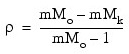
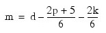
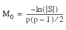
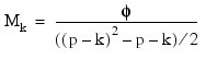
Where:
|S| is the determinant of Covariances
p = N_ELEMENTS(Covariances(0, *))
k = N_ELEMENTS(Covariances(0, *))
φ is the optimized criterion
d = Df
Image Analysis
The term image analysis is used here to denote the noniterative image method of Kaiser (1963), rather than the image analysis discussed by Harman (1976, p. 226). The image method (as well as the alpha-factor analysis method) begins with the notion that only a finite number from an infinite number of possible variables have been measured. The image-factor pattern is calculated under the assumption that the ratio of the number of factors to the number of observed variables is near zero, so that a very good estimate for the unique error variances (for standardized variables) is given as 1 minus the squared multiple correlation of the variable under consideration with all variables in the covariance matrix.
First, the matrix D2 = (diag(S–1))–1 is computed, where the operator diag results in a matrix consisting of the diagonal elements of its argument and S is the sample covariance (correlation) matrix. Then, the eigenvalues Λ and eigenvectors Γ of the matrix D –1SD–1 are computed. Finally, the unrotated image-factor pattern is computed as DΓ [ ( Λ – I )2 Λ–1 ]1/2.
Alpha-factor Analysis
The alpha-factor analysis method of Kaiser and Caffrey (1965) finds factor-loading estimates to maximize the correlation between the factors and the complete universe of variables of interest. The basic idea in this method is that only a finite number of variables out of a much larger set of possible variables is observed. The population factors are linearly related to this larger set, while the observed factors are linearly related to the observed variables. Let f denote the factors obtainable from a finite set of observed random variables, and let ξ denote the factors obtainable from the universe of observable variables. Then, the alpha method attempts to find factor-loading estimates so as to maximize the correlation between f and ξ. In order to obtain these estimates, the iterative algorithm of Kaiser and Caffrey (1965) is used.
Comments
- IMSL_FACTOR_ANALYSIS makes no attempt to solve for N_factors. In general, if N_factors is not known in advance, several different values should be used and the most reasonable value kept in the final solution.
- Iterative methods are generally thought to be superior from a theoretical point of view, but in practice, often lead to solutions that differ little from the noniterative methods. For this reason, it is usually suggested that a noniterative method be used in the initial stages of the factor analysis and that the iterative methods be used when issues such as the number of factors have been resolved.
- Initial estimates for the unique variances can be input. If the iterative methods fail for these values, new initial estimates should be tried. These can be obtained by use of another factoring method. (Use the final estimates from the new method as the initial estimates in the old method.)
Examples
Example 1
In this example, factor analysis is performed for a nine-variable matrix using the default method of unweighted least squares.
covariances = $
[[1.0, 0.523, 0.395, 0.471, 0.346, 0.426, 0.576, 0.434, 0.639], $
[0.523, 1.0, 0.479, 0.506, 0.418, 0.462, 0.547, 0.283, 0.645], $
[0.395, 0.479, 1.0, 0.355, 0.27, 0.254, 0.452, 0.219, 0.504], $
[0.471, 0.506, 0.355, 1.0, 0.691, 0.791, 0.443, 0.285, 0.505], $
[0.346, 0.418, 0.27, 0.691, 1.0, 0.679, 0.383, 0.149, 0.409], $
[0.426, 0.462, 0.254, 0.791, 0.679, 1.0, 0.372, 0.314, 0.472], $
[0.576, 0.547, 0.452, 0.443, 0.383, 0.372, 1.0, 0.385, 0.68], $
[0.434, 0.283, 0.219, 0.285, 0.149, 0.314, 0.385, 1.0, 0.47], $
[0.639, 0.645, 0.504, 0.505, 0.409, 0.472, 0.68, 0.47, 1.0]]
n_factors = 3
a = IMSL_FACTOR_ANALYSIS(covariances, n_factors)
PM, a, Title = 'Unrotated Loadings:'
IDL prints:
Unrotated Loadings:
0.701801 -0.231594 0.0795559
0.719964 -0.137227 -0.208225
0.535122 -0.214389 -0.22709
0.790669 0.405017 0.00704257
0.653203 0.422066 -0.104563
0.753915 0.484247 0.160720
0.712674 -0.281911 -0.0700779
0.483540 -0.262720 0.461992
0.819210 -0.313728 -0.0198735
Example 2
The following data were originally analyzed by Emmett (1949). There are 211 observations on nine variables. Following Lawley and Maxwell (1971), three factors are obtained by the method of maximum likelihood. This example uses the same data as the first example.
n_factors = 3
a = IMSL_FACTOR_ANALYSIS(covariances, n_factors, $
Max_Likelihood=210, Switch_Eps=0.01, $
Eps=0.000001, Itmax=30, Max_Steps=10)
PM, a, Title = 'Unrotated Loadings:'
IDL prints:
Unrotated Loadings:
0.664210 -0.320874 0.0735207
0.688833 -0.247138 -0.193280
0.492616 -0.302161 -0.222433
0.837198 0.292427 -0.0353954
0.705002 0.314794 -0.152784
0.818701 0.376672 0.104524
0.661494 -0.396031 -0.0777453
0.457925 -0.295526 0.491347
0.765668 -0.427427 -0.0116992
Errors
Warning Errors
STAT_VARIANCES_INPUT_IGNORED: When using the keyword PRINC_COMP, the unique variances are assumed to be zero. Input for UNIQUE_VAR_IN is ignored.
STAT_TOO_MANY_ITERATIONS: Too many iterations. Convergence is assumed.
STAT_NO_DEG_FREEDOM: No degrees of freedom for the significance testing.
STAT_TOO_MANY_HALVINGS: Too many step halvings. Convergence is assumed.
Fatal Errors
STAT_HESSIAN_NOT_POS_DEF: Approximate Hessian is not semidefinite on iteration #. The computations cannot proceed. Try using different initial estimates.
STAT_FACTOR_EVAL_NOT_POS: Variable EIGENVALUES(#) = #. An eigenvalue corresponding to a factor is negative or zero. Either use different initial estimates for UNIQUE_VAR_IN or reduce the number of factors.
STAT_COV_NOT_POS_DEF: Parameter covariances is not positive semidefinite. The computations cannot proceed.
STAT_COV_IS_SINGULAR: Matrix covariances is singular. The computations cannot continue because variable # is linearly related to the remaining variables.
STAT_COV_EVAL_ERROR: An error occurred in calculating the eigenvalues of the adjusted (inverse) covariance matrix. Check Covariances.
STAT_ALPHA_FACTOR_EVAL_NEG: In alpha-factor analysis on iteration #, eigenvalue # is #. As all eigenvalues corresponding to the factors must be positive, either the number of factors must be reduced or new initial estimates for UNIQUE_VAR_IN must be given.
Syntax
Result = IMSL_FACTOR_ANALYSIS(Covariances, N_factors [, ALPHA=value] [, CHI_SQ_TEST=variable] [, /DOUBLE] [, EIGENVALUES=variable] [, EPS=value] [, F_MIN=variable] [, /GEN_LSQ] [, /IMAGE] [, ITERS=variable] [, ITMAX=value] [, LAST_STEP=variable] [, MAX_LIKELIHOOD=value] [, MAX_STEPS=value] [, /PRINC_COMP] [, /PRINC_FACTOR] [, SWITCH_EPS=value] [, TUCKER_COEF=variable] [, UNIQUE_VAR_IN=array] [, UNIQUE_VAR_OUT=array] [, /UNWGT_LSQ])
Return Value
A two-dimensional array containing the matrix of factor loadings.
Arguments
Covariances
Two-dimensional array containing the variance-covariance or correlation matrix.
N_factors
Number of factors in the model.
Keywords
ALPHA (optional)
The number of degrees of freedom in covariances. Using ALPHA forces the alpha-factor analysis (common factor model) method to be used to obtain the estimates.
CHI_SQ_TEST (optional)
Named variable in the form of a one-dimensional array of length 3 containing the chi- squared test statistics. The contents of the array are, in order, the number of degrees of freedom in chi-squared, the chi-squared test statistic for testing that N_factors common factors are adequate for the data, and the probability of a greater chi-squared statistic.
DOUBLE (optional)
If present and nonzero, double precision is used.
EIGENVALUES (optional)
Named variable into which a one-dimensional array of length N_ELEMENTS(Covariances(0, *)) containing the eigenvalues of the matrix from which the factors were extracted is stored.
EPS (optional)
Convergence criterion used to terminate the iterations. For the unweighted least squares, generalized least squares, or maximum likelihood methods, convergence is assumed when the relative change in the criterion is less than EPS. For alpha-factor analysis, convergence is assumed when the maximum change (relative to the variance) of a uniqueness is less than EPS. The default value is 0.0001.
F_MIN (optional)
Named variable into which the value of the function minimum is stored.
GEN_LSQ (optional)
If present and nonzero, the generalized least-squares (common factor model) method is used to obtain the estimates. MAX_LIKELIHOOD, PRINC_COMP, PRINC_FACTOR, UNWGT_LSQ, GEN_LSQ, IMAGE, and ALPHA cannot be used together.
IMAGE (optional)
If present and nonzero, the image-factor analysis (common factor model) method is used to obtain the estimates. MAX_LIKELIHOOD, PRINC_COMP, PRINC_FACTOR, UNWGT_LSQ, GEN_LSQ, IMAGE, and ALPHA cannot be used together.
ITERS (optional)
Named variable into which the number of iterations is stored.
ITMAX (optional)
Maximum number of iterations in the iterative procedure. The default value is 60.
LAST_STEP (optional)
Named variable in the form of an array of length N_ELEMENTS(Covariances(0, *)). The array contains the updates of the unique variance estimates when convergence was reached (or the iterations terminated).
MAX_LIKELIHOOD (optional)
The number of degrees of freedom in covariances. Using Max_Likelihood forces the maximum likelihood (common factor) model to be used to obtain the estimates. MAX_LIKELIHOOD, PRINC_COMP, PRINC_FACTOR, UNWGT_LSQ, GEN_LSQ, IMAGE, and ALPHA cannot be used together.
MAX_STEPS (optional)
Maximum number of step halvings allowed during any one iteration. The default value is 10.
PRINC_COMP (optional)
If present and nonzero, the principal component (principal component model) is used to obtain the estimates.
PRINC_FACTOR
If present and nonzero, the principal factor (common factor model) is used to obtain the estimates. MAX_LIKELIHOOD, PRINC_COMP, PRINC_FACTOR, UNWGT_LSQ, GEN_LSQ, IMAGE, and ALPHA cannot be used together.
SWITCH_EPS (optional)
Convergence criterion used to switch to exact second derivatives. When the largest relative change in the unique standard deviation vector is less than SWITCH_EPS, exact second derivative vectors are used. The value of SWITCH_EPS is not used with the principal component, principal factor, image-factor analysis, or alpha-factor analysis methods. The default value is 0.1.
TUCKER_COEF (optional)
Named variable into which the Tucker reliability coefficient is stored.
UNIQUE_VAR_IN (optional)
One-dimensional array of length N_ELEMENTS(Covariances(0, *)) containing the initial estimates of the unique variances. Default: initial estimates are taken as the constant 1 – N_factors/2 * N_ELEMENTS(Covariances(0, *)) divided by the diagonal elements of the inverse of covariances.
UNIQUE_VAR_OUT (optional)
One-dimensional array of length N_ELEMENTS(Covariances(0, *)) containing the estimated unique variances.
UNWGT_LSQ (optional)
If present and nonzero, the unweighted least-squares (common factor model) method is used to obtain the estimates. This option is the default. MAX_LIKELIHOOD, PRINC_COMP, PRINC_FACTOR, UNWGT_LSQ, GEN_LSQ, IMAGE, and ALPHA cannot be used together.
Version History