The IMSL_FFTCOMP function computes the discrete Fourier transform of a real or complex sequence. Using keywords, a real-to-complex transform or a two- dimensional complex Fourier transform can be computed.
This routine requires an IDL Advanced Math and Stats license. For more information, contact your sales or technical support representative.
The IMSL_FFTCOMP function’s default action is to compute the FFT of array A, with the type of FFT performed dependent upon the data type of the input array A. (If A is a one-dimensional real array, the real FFT is computed; if A is a one-dimensional complex array, the complex FFT is computed; and if A is a two-dimensional real or complex array, the complex FFT is computed.) If the complex FFT of a one-dimensional real array is desired, the keyword COMPLEX should be specified. The keywords SINE and COSINE allow IMSL_FFTCOMP to be used to compute the discrete Fourier sine or cosine transformation of a one dimensional real array. The remainder of this section is divided into separate discussions of the various uses of IMSL_FFTCOMP.
Case 1: One-dimensional Real FFT
If A is one-dimensional and real, the IMSL_FFTCOMP function computes the discrete Fourier transform of a real array of length n = N_ELEMENTS (A). The method used is a variant of the Cooley-Tukey algorithm, which is most efficient when n is a product of small prime factors. If n satisfies this condition, then the computational effort is proportional to nlogn.
By default, IMSL_FFTCOMP computes the forward transform. If n is even, the forward transform is as follows:
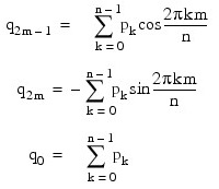
If n is odd, qm is defined as above for m from 1 to (n – 1) / 2.
Let f be a real-valued function of time. Suppose f is sampled at n equally spaced time intervals of length ∆ seconds starting at time t0:
pi = f(t0 + i∆) i = 0, 1, ..., n – 1
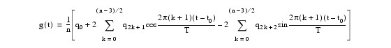
Assume that n is odd for the remainder of the discussion for the case in which A is real. The IMSL_FFTCOMP function treats this sequence as if it were periodic of period n. In particular, it assumes that f(t0) = f(t0 + n∆). Hence, the period of the
function is assumed to be T = n∆. The above transform is inverted for the following:

This formula can be interpreted in the following manner: The coefficients q produced by IMSL_FFTCOMP determine an interpolating trigonometric polynomial to the data. That is, if the equations are defined as:
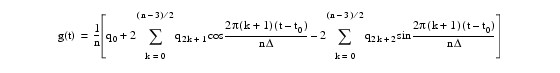
then the result is as follows:
f(t0 + i∆ ) = g(t0 + i∆ )
Now suppose the dominant frequencies are to be obtained. Form the array P of length (n + 1) / 2 as follows:

These numbers correspond to the energy in the spectrum of the signal. In particular, Pk corresponds to the energy level at the following frequency:

Furthermore, note that there are only:

resolvable frequencies when n observations are taken. This is related to the Nyquist phenomenon, which is induced by discrete sampling of a continuous signal. Similar relations hold for the case when n is even.
If the keyword BACKWARD is specified, the backward transform is computed. If n is even, the backward transform is as follows:

If n is odd, the following is true:

The backward Fourier transform is the unnormalized inverse of the forward Fourier transform.
IMSL_FFTCOMP is based on the real FFT in FFTPACK, which was developed by Paul Swarztrauber at the National Center for Atmospheric Research.
Case 2: One-dimensional Complex FFT
If A is one-dimensional and complex, the IMSL_FFTCOMP function computes the discrete Fourier transform of a complex array of size n = N_ELEMENTS (a). The method used is a variant of the Cooley Tukey algorithm, which is most efficient when n is a product of small prime factors. If n satisfies this condition, the computational effort is proportional to nlogn.
By default, IMSL_FFTCOMP computes the forward transform as in the equation below:
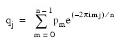
Note, the Fourier transform can be inverted as follows:

This formula reveals the fact that, after properly normalizing the Fourier coefficients, you have coefficients for a trigonometric interpolating polynomial to the data.
If the keyword BACKWARD is used, the following computation is performed:

Furthermore, the relation between the forward and backward transforms is that they are unnormalized inverses of each other. In other words, the following code fragment begins with an array p and concludes with an array p2 = np:
q = IMSL_FFTCOMP(p)
p2 = IMSL_FFTCOMP(q, /Backward)
Case 3: Two-dimensional FFT
If A is two-dimensional and real or complex, the IMSL_FFTCOMP function computes the discrete Fourier transform of a two-dimensional complex array of size n x m where n = N_ELEMENTS (a (*, 0)) and m = N_ELEMENTS (a (0, *)). The method used is a variant of the Cooley-Tukey algorithm, which is most efficient when both n and m are a product of small prime factors. If n and m satisfy this condition, then the computational effort is proportional to nmlognm.
By default, given a two-dimensional array, IMSL_FFTCOMP computes the forward transform as in the following equation:

Note, the Fourier transform can be inverted as follows:

This formula reveals the fact that, after properly normalizing the Fourier coefficients, you have the coefficients for a trigonometric interpolating polynomial to the data.
If the keyword BACKWARD is used, the following computation is performed:

Case 4: Cosine Transform of a Real Sequence
If the keyword COSINE is present and nonzero, the IMSL_FFTCOMP function computes the discrete Fourier cosine transform of a real vector of size N. The method used is a variant of the Cooley-Tukey algorithm, which is most efficient when N – 1 is a product of small prime factors. If N satisfies this condition, then the computational effort is proportional to NlogN. Specifically, given an N-vector p, IMSL_FFTCOMP returns in q:

where p = array a and q = result.
Finally, note that the Fourier cosine transform is its own (unnormalized) inverse.
Case 5: Sine Transform of a Real Sequence
If the keyword SINE is present and nonzero, the IMSL_FFTCOMP function computes the discrete Fourier sine transform of a real vector of size N. The method used is a variant of the Cooley-Tukey algorithm, which is most efficient when N + 1 is a product of small prime factors. If N satisfies this condition, then the computational effort is proportional to NlogN. Specifically, given an N-vector p, IMSL_FFTCOMP returns in q:

where p = array a and q = result.
Finally, note that the Fourier sine transform is its own (unnormalized) inverse.
Examples
Example 1
This example uses a pure cosine wave as a data array, and its Fourier series is recovered. The Fourier series is an array with all components zero except at the appropriate frequency where it has an n/2.
n = 7
p = COS(FINDGEN(n) * 2 * !Pi/n)
PM, p
IDL prints:
1.00000
0.623490
-0.222521
-0.900969
-0.900969
-0.222521
0.623490
Continue:
q = IMSL_FFTCOMP(p)
PM, q, FORMAT = '(f8.3)'
IDL prints:
0.000
3.500
0.000
-0.000
-0.000
0.000
-0.000
Example 2: Resolving Dominant Frequencies
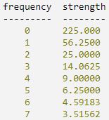
The following procedure demonstrates how the FFT can be used to resolve the dominant frequency of a signal. Call IMSL_FFTCOMP with a data vector of length n = 15, filled with pure, exponential signals of increasing frequency and decreasing strength. Using the computed FFT, the relative strength of the frequencies is resolved. It is important to note that for an array of length n, at most (n + 1)/2 frequencies can be resolved using the computed FFT.
.RUN
PRO power_spectrum
n = 15
num_freq = n/2 + (n MOD 2)
z = COMPLEX(0, FINDGEN(n) * 2 * !Pi/n)
p = COMPLEXARR(n)
FOR i = 0, num_freq - 1 DO p = p + EXP(i * z)/(i + 1)
q = IMSL_FFTCOMP(p)
power = FLTARR(num_freq)
IF ((n MOD 2) EQ 0) THEN BEGIN
power(0) = ABS(q(0))^2
FOR i = 1,(num_freq - 2) DO $
power(i) = q(i) * CONJ(q(i)) + q(n-i-1) * CONJ(q(n-i-1))
power(num_freq - 1)=q(num_freq - 1)*CONJ(q(num_freq - 1))
ENDIF
IF ((n MOD 2) EQ 1) THEN BEGIN
FOR i = 1,(num_freq - 1) DO power(i) = $
q(i)^2 + q(n - i)^2 power(0) = q(0)^2
ENDIF
PRINT, ' frequency strength' & $
PRINT, ' --------- --------' & $
FOR i = 0,7 DO PRINT, i, power(i)
END
IDL prints:
Example 3: Computing a Two-dimensional FFT
This example computes the forward transform of a two-dimensional matrix followed by the backward transform. Notice that the process of computing the forward transform followed by the backward transform multiplies the entries of the original matrix by the product of the lengths of the two dimensions.
n = 4
m = 5
p = COMPLEXARR(n, m)
FOR i = 0, n - 1 DO BEGIN & $
z = COMPLEX(0, 2 * i * 2 * !Pi/n) & $
FOR j = 0, m - 1 DO BEGIN & $
w = COMPLEX(0, 5 * j * 2 * !Pi/m) & $
p(i, j) = EXP(z) * EXP(w) & $
ENDFOR & $
ENDFOR
q = IMSL_FFTCOMP(p)
p2 = IMSL_FFTCOMP(q, /Backward)
FORMAT = '(4("(",f6.2,",",f5.2,")",2x))'
PM, p, FORMAT = format, TITLE = 'p'
IDL prints:
p
( 1.0, 0.0)( 1.0, 0.0)( 1.0, 0.0)( 1.0, 0.0)
( 1.0, 0.0)(-1.0,-0.0)(-1.0,-0.0)(-1.0,-0.0)
(-1.0,-0.0)(-1.0,-0.0)( 1.0, 0.0)( 1.0, 0.0)
( 1.0, 0.0)( 1.0, 0.0)( 1.0, 0.0)(-1.0,-0.0)
(-1.0,-0.0)(-1.0,-0.0)(-1.0,-0.0)(-1.0,-0.0)
PM, q, FORMAT = format, TITLE = 'q = IMSL_FFTCOMP(p)' q = IMSL_FFTCOMP(p)
IDL prints:
( 0.0, 0.0)(-0.0, 0.0)( 0.0, 0.0)(-0.0, 0.0)
( 0.0, 0.0)(-0.0,-0.0)( 0.0,-0.0)( 0.0,-0.0)
( 0.0, 0.0)(-0.0, 0.0)(20.0, 0.0)(-0.0,-0.0)
(-0.0,-0.0)( 0.0,-0.0)( 0.0,-0.0)( 0.0,-0.0)
( 0.0, 0.0)(-0.0, 0.0)(-0.0,-0.0)(-0.0,-0.0)
PM, p2, FORMAT = format, TITLE = 'p2 = IMSL_FFTCOMP(q, /BACKWARD)'
p2 = IMSL_FFTCOMP(q, /Backward)
IDL prints:
( 20., 0.)( 20., 0.)( 20., 0.)( 20., 0.)
( 20., 0.)(-20.,-0.)(-20.,-0.)(-20.,-0.)
(-20.,-0.)(-20.,-0.)( 20., 0.)( 20., 0.)
( 20., 0.)( 20., 0.)( 20., 0.)(-20.,-0.)
(-20.,-0.)(-20.,-0.)(-20.,-0.)(-20.,-0.)
Syntax
Result = IMSL_FFTCOMP(A [, COSINE=value] [, SINE=value] [, /DOUBLE] [, COMPLEX=value] [, BACKWARD=value] [, INIT_PARAMS=array])
Return Value
Two-dimensional array of size nx by ny containing solution at the grid points.
Arguments
A
Array containing the periodic sequence.
Keywords
BACKWARD (optional)
If present and nonzero, the backward transform is computed. See the discussion above for more details on this option.
COMPLEX (optional)
If present and nonzero, the complex transform is computed. If A is complex, this keyword is not required to ensure that a complex transform is computed. If A is real, it is promoted to complex internally.
COSINE (optional)
If present and nonzero, then IMSL_FFTCOMP computes the discrete Fourier cosine transformation of an even sequence.
DOUBLE (optional)
If present and nonzero, then double precision is used.
INIT_PARAMS (optional)
Array containing parameters used when computing a one-dimensional FFT. If IMSL_FFTCOMP is used repeatedly with arrays of the same length and data type, it is more efficient to compute these parameters only once with a call to the IMSL_FFTINIT function.
SINE (optional)
If present and nonzero, then IMSL_FFTCOMP computes the discrete Fourier sine transformation of an odd sequence.
Version History