The IMSL_LNORMREGRESS function fits a multiple linear regression model using criteria other than least squares. Namely, IMSL_LNORMREGRESS allows you to choose Least Absolute Value (L1), Least Lp norm (Lp), or Least Maximum Value (Minimax or Linfinity) method of multiple linear regression.
This routine requires an IDL Advanced Math and Stats license. For more information, contact your sales or technical support representative.
Least Absolute Value Criterion
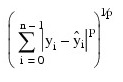
The IMSL_LNORMREGRESS function computes estimates of the regression coefficients in a multiple linear regression model. For keyword LAV (default), the criterion satisfied is the minimization of the sum of the absolute values of the deviations of the observed response yi from the fitted response:

for a set on n observations. Under this criterion, known as the L1 or LAV (least absolute value) criterion, the regression coefficient estimates minimize:

The estimation problem can be posed as a linear programming problem. The special nature of the problem, however, allows for considerable gains in efficiency by the modification of the usual simplex algorithm for linear programming. These modifications are described in detail by Barrodale and Roberts (1973, 1974).
In many cases, the algorithm can be made faster by computing a least-squares solution prior to the use of keyword Lav. This is particularly useful when a least- squares solution has already been computed. The procedure is as follows:
- Fit the model using least squares and compute the residuals from this fit.
- Fit the residuals from Step 1 on the regressor variables in the model using keyword Lav.
- Add the two estimated regression coefficient vectors from Steps 1 and 2. The result is an L1 solution.
When multiple solutions exist for a given problem, option LAV may yield different estimates of the regression coefficients on different computers, however, the sum of the absolute values of the residuals should be the same (within rounding differences). The informational error indicating nonunique solutions may result from rounding accumulation. Conversely, because of rounding the error may fail to result even when the problem does have multiple solutions.
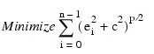
Lp Norm Criterion
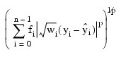
Keyword LLP computes estimates of the regression coefficients in a multiple linear regression model y = Xβ + ε under the criterion of minimizing the Lp norm of the deviations for i = 0, ... , n - 1 of the observed responseyi from the fitted response:
for a set on n observations and for p ≥ 1. For the case when keywords WEIGHTS and FREQUENCIES are not supplied, the estimated regression coefficient vector:
βˆ
(output in Result) minimizes the Lp norm:
The choice p = 1 yields the maximum likelihood estimate for β when the errors have a Laplace distribution. The choice p = 2 is best for errors that are normally distributed. Sposito (1989, pages 36−40) discusses other reasonable alternatives for p based on the sample kurtosis of the errors.
Weights are useful if errors in the model have known unequal variances:

In this case, the weights should be taken as:

Frequencies are useful if there are repetitions of some observations in the data set. If a single row of data corresponds to ni observations, set the frequency fi =ni. In general, keyword Llp minimizes the Lp norm:
The asymptotic variance-covariance matrix of the estimated regression coefficients is given by:

where R is from the QR decomposition of the matrix of regressors (output in keyword R_MATRIX) and where an estimate of λ2 is output in keyword SCALE.
In the discussion that follows, we will first present the algorithm with frequencies and weights all taken to be one. Later, we will present the modifications to handle frequencies and weights different from one.
Keyword LLP uses Newton’s method with a line search for p > 1.25 and, for p ≤ 1.25, uses a modification due to Ekblom (1973, 1987) in which a series of perturbed problems are solved in order to guarantee convergence and increase the convergence rate. The cutoff value of 1.25 as well as some of the other implementation details given in the remaining discussion were investigated by Sallas (1990) for their effect on CPU times.
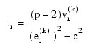
For the first iteration in each case, a least-squares solution for regression coefficients is computed with IMSL_MULTIREGRESS. If p = 2, the computations are finished. Otherwise, the residuals from the k-th iteration:

are used to compute the gradient and Hessian for the Newton step for the (k + 1)-st iteration for minimizing the p-th power of the Lp norm. (The exponent 1/p in the Lp norm can be omitted during the iterations.)
For subsequent iterations, we first discuss the p > 1.25 case. For p > 1.25, the gradient and Hessian at the (k + 1)-st iteration depend upon:

and:

In the case 1.25 < p < 2 and:

and the Hessian are undefined; and we follow the recommendation of Merle and Spath (1974). Specifically, we modify the definition of:

to the following:
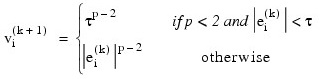
where τ equals 100 * machine epsilon times the square root of the residual mean square from the least-squares fit.
Let V(k+1) be a diagonal matrix with diagonal entries:

and let z(k+1) be a vector with elements:

In order to compute the step on the (k + 1)-st iteration, the R from the QR decomposition of:
[V(k+1)]1/2X
is computed using fast Givens transformations. Let:
R(k+1)
denote the upper triangular matrix from the QR decomposition. The linear system:
[R(k+1)]TR(k+1)d(k+1) = XT z(k+1)
is solved for:
d(k+1)
where R(k+1) is from the QR decomposition of [V(k+1)]1/2X. The step taken on the (k + 1)-st iteration is:

The first attempted step on the (k + 1)-st iteration is with α(k+1) = 1. If all of the:

are nonzero, this is exactly the Newton step. See Kennedy and Gentle (1980, pages 528−529) for further discussion.
If the first attempted step does not lead to a decrease of at least one-tenth of the predicted decrease in the p-th power of the Lp norm of the residuals, a backtracking linesearch procedure is used. The backtracking procedure uses a one-dimensional quadratic model to estimate the backtrack constant p. The value of p is constrained to be no less that 0.1. An approximate upper bound for p is 0.5. If after 10 successive backtrack attempts, α(k) = p1p2... p10 does not produce a step with a sufficient decrease, then IMSL_LNORMREGRESS issues a message with error code 5. For further details on the backtrack line-search procedure, see Dennis and Schnabel (1983, pages 126−127).
Convergence is declared when the maximum relative change in the residuals from one iteration to the next is less than or equal to EPS. The relative change:

in the i-th residual from iteration k to iteration k + 1 is computed as follows:
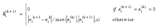
where s is the square root of the residual mean square from the least-squares fit on the first iteration.
For the case 1 ≤ p ≤ 1.25, we describe the modifications to the previous procedure that incorporate Ekblom’s (1973) results. A sequence of perturbed problems are solved with a successively smaller perturbation constant c. On the first iteration, the least-squares problem is solved. This corresponds to an infinite c. For the second problem, c is taken equal to s, the square root of the residual mean square from the least- squares fit. Then, for the (j + 1)-st problem, the value of c is computed from the previous value of c according to:
Each problem is stated as:
For each problem, the gradient and Hessian on the (k + 1)-st iteration depend upon:

and:

where:

The linear system [R(k+1)]TR(k+1)d(k+1) = XTz(k+1) is solved for d(k+1) where R(k+1) is from the QR decomposition of [V(k+1)]1/2X. The step taken on the (k + 1)-st iteration is:

where the first attempted step is with α(k+1) = 1. If necessary, the backtracking line- search procedure discussed earlier is used.
Convergence for each problem is relaxed somewhat by using a convergence epsilon equal to max(EPS, 10–j) where j = 1, 2, 3, ... indexes the problems (j = 0 corresponds to the least-squares problem).
After the convergence of a problem for a particular c, Ekblom’s (1987) extrapolation technique is used to compute the initial estimate of β for the new problem. Let R(k):

and c be from the last iteration of the last problem. Let:
and let t be the vector with elements ti. The initial estimate of β for the new problem with perturbation constant 0.01c is:

where ∆c = (0.01c - c) = -0.99c, and where d is the solution of the linear system [R(k)]TR(k)d = XTt.
Convergence of the sequence of problems is declared when the maximum relative difference in residuals from the solution of successive problems is less than EPS.
The preceding discussion was limited to the case for which WEIGHTS(*) = 1 and FREQUENCIES(*) = 1, i.e., the weights and frequencies are all taken equal to one. The necessary modifications to the preceding algorithm to handle weights and frequencies not all equal to one are as follows:
1. Replace:

in the definitions of:

and ti.
2. Replace:

These replacements have the same effect as multiplying the i-th row of X and y by:

and repeating the row fi times except for the fact that the residuals returned by IMSL_LNORMREGRESS are in terms of the original y and X.
Finally, R and an estimate of λ2 are computed. Actually, R is recomputed because on output it corresponds to the R from the initial QR decomposition for least squares. The formula for the estimate of λ2 depends on p.
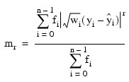
For p = 1, the estimator for λ2 is given by (McKean and Schrader 1987):
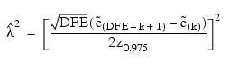
with:

where z0.975 is the 97.5 percentile of standard normal distribution, and:

are ordered residuals where Rank zero residuals are excluded. Note that:
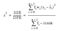
For p = 2, the estimator of λ2 is the customary least-squares estimator given by:
For 1 < p < 2 and for p > 2, the estimator for λ2 is given by (Gonin and Money 1989):

with:
Least Minimum Value Criterion (minimax)
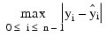
Keyword LMV computes estimates of the regression coefficients in a multiple linear regression model. The criterion satisfied is the minimization of the maximum deviation of the observed response yi from the fitted response:
for a set on n observations. Under this criterion, known as the minimax or LMV (least maximum value) criterion, the regression coefficient estimates minimize:
The estimation problem can be posed as a linear programming problem. A dual simplex algorithm is appropriate, however, the special nature of the problem allows for considerable gains in efficiency by modification of the dual simplex iterations so as to move more rapidly toward the optimal solution. The modifications are described in detail by Barrodale and Phillips (1975).
When multiple solutions exist for a given problem, LMV may yield different estimates of the regression coefficients on different computers, however, the largest residual in absolute value should have the same absolute value (within rounding differences). The informational error indicating nonunique solutions may result from rounding accumulation. Conversely, because of rounding, the error may fail to result even when the problem does have multiple solutions.
Examples
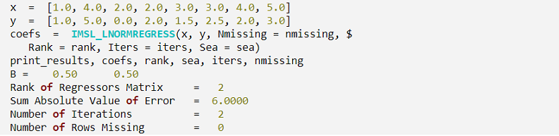
Example 1
A straight line fit to a data set is computed under the LAV criterion.
PRO print_results, coefs, rank, sea, iters, nmissing
PRINT, 'B = ', coefs(0), coefs(1), $
FORMAT = '(A6, F5.2, 5X, F5.2)'
PRINT
PRINT, 'Rank of Regressors Matrix = ', rank, $
FORMAT = '(A32, I3)'
PRINT, 'Sum Absolute Value of Error = ', sea, $
FORMAT = '(A32, F7.4)'
PRINT, 'Number of Iterations = ', iters, $
FORMAT = '(A32, I3)'
PRINT, 'Number of Rows Missing = ', nmissing, $
FORMAT = '(A32, I3)'
END
IDL prints:
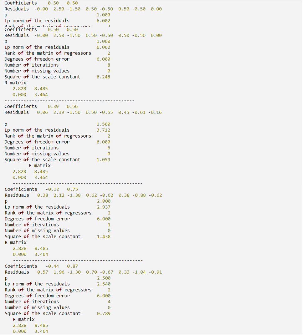
Example 2
Different straight line fits to a data set are computed under the criterion of minimizing the Lp norm by using p equal to 1, 1.5, 2.0 and 2.5.
.RUN
PRO print_results, coefs, residuals, p, resid_norm, rank, df, $
iters, nmissing, scale, rm
PRINT, 'Coefficients ', coefs, FORMAT = '(A13, 2F7.2)' PRINT, 'Residuals ', residuals, FORMAT = '(A10, 8F6.2)' PRINT
PRINT, 'p ', p, $ FORMAT = '(A33, F6.3)'
PRINT, 'Lp norm of the residuals ', resid_norm, $
FORMAT = '(A33, F6.3)'
PRINT, 'Rank of the matrix of regressors ', rank, $ FORMAT = '(A33, I6)'
PRINT, 'Degrees of freedom error ', df, $ FORMAT = '(A33, F6.3)'
PRINT, 'Number of iterations ', iters, $
FORMAT = '(A33, I6)'
PRINT, 'Number of missing values ', nmissing, $ FORMAT = '(A33, I6)'
PRINT, 'Square of the scale constant ', scale, $ FORMAT = '(A33, F6.3)'
PRINT
PM, rm, FORMAT = '(2F8.3)', Title = ' R matrix' PRINT
PRINT, '------------------------------------------------'
PRINT
END
.RUN
x = [1.0, 4.0, 2.0, 2.0, 3.0, 3.0, 4.0, 5.0]
y = [1.0, 5.0, 0.0, 2.0, 1.5, 2.5, 2.0, 3.0]
eps = 0.001
FOR i = 0, 3 DO BEGIN
p = 1.0 + i*0.5
coefs = IMSL_LNORMREGRESS(x, y, /Llp, P = p, Eps = eps, $
Nmissing = nmissing, Rank = rank, $
Iters = iters, Scale = scale, $
Df = df, R_Matrix = rm, Residuals = residuals, $
Resid_Norm = resid_norm)
print_results, coefs, residuals, p, resid_norm, rank, df, $
iters, nmissing, scale, rm
ENDFOR
END
IDL prints:
Example 3
A straight line fit to a data set is computed under the LMV criterion.
.RUN
PRO print_results, coefs, rank, rm, iters, nmissing
PRINT, 'B = ', coefs(0), coefs(1), $
FORMAT = '(A6, F5.2, 5X, F5.2)'
PRINT
PRINT, 'Rank of Regressors Matrix = ', rank, $
FORMAT = '(A34, I3)'
PRINT, 'Magnitude of Largest Residual = ', rm, $
FORMAT = '(A34, F7.4)'
PRINT, 'Number of Iterations = ', iters, $
FORMAT = '(A34, I3)'
PRINT, 'Number of Rows Missing = ', nmissing, $
FORMAT = '(A34, I3)'
END
IDL prints:
Syntax
Result = IMSL_LNORMREGRESS(X, Y [, DF=variable] [, /DOUBLE] [, EPS=value] [, FREQUENCIES=array] [, ITERS=variable] [, /LAV | /LLP | /LMV] [, NMISSING=variable] [, /NO_INTERCEPT] [, P=value] [, RANK=variable] [, R_MATRIX=variable] [, RESID_MAX=variable] [, RESID_NORM=variable] [, RESIDUALS=variable] [, SCALE=variable] [, SEA=variable] [, TOLERANCE=value] [, WEIGHTS=array])
Return Value
One-dimensional array of length n_independent + 1 containing a least absolute value solution for the regression coefficients. The estimated intercept is the initial component of the array, where the i-th component contains the regression coefficients for the i-th dependent variable. If the keyword No_Intercept is used then the (i-1)-st component contains the regression coefficients for the i-th dependent variable. IMSL_LNORMREGRESS returns the Lp norm or least maximum value solution for
the regression coefficients when appropriately specified in the input keyword list.
Arguments
X
Two-dimensional array of size n_rows by n_independent containing the independent (explanatory) variables(s) where n_rows = N_ELEMENTS(x(*,0)) and n_independent is the number of independent (explanatory) variables. The i-th column of x contains the i-th independent variable.
Y
One-dimensional array of size n_rows containing the dependent (response) variable.
Keywords
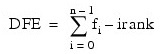
DF (optional)
Named variable into which the sum of the frequencies minus Rank is stored. In least squares fit (p=2) Df is called the degrees of freedom of error. Keyword LLP is required when using keyword DF.
DOUBLE (optional)
If present and nonzero, double precision is used.
EPS (optional)
Convergence criterion. If the maximum relative difference in residuals from the k-th to (k+1)-st iterations is less than EPS, convergence is declared. Keyword LLP is required when using keyword EPS. Default: 100 * (machine epsilon).
FREQUENCIES (optional)
One-dimensional array of size n_rows containing the frequencies for the independent (explanatory) variable. Keyword LLP is required when using keyword FREQUENCIES.
ITERS (optional)
Named variable into which the number of iterations performed is stored.
LAV (optional)
By default (or if LAV is used) the function fits a multiple linear regression model using the least absolute values criterion. Keywords LAV, LLP, and LMV can not be used together.
LLP (optional)
If present and nonzero, IMSL_LNORMREGRESS fits a multiple linear regression model using the Lp norm criterion. LLP requires the keyword P, for P ≥ 1. Keywords Lav, Llp, and Lmv can not be used together.
LMV (optional)
If present and nonzero, IMSL_LNORMREGRESS fits a multiple linear regression model using the minimax criterion. Keywords Lav, Llp, and Lmv cannot be used together.
NMISSING (optional)
Named variable into which the number of rows of data containing NaN (not a number) for the dependent or independent variables is stored. If a row of data contains NaN for any of these variables, that row is excluded from the computations.
NO_INTERCEPT (optional)
If present and nonzero, the intercept term:
βˆ 0
is omitted from the model and the return value from regression is a one-dimensional array of length n_independent. By default the fitted value for observation i is:
βˆ 0 + βˆ 1 x1 + ... + βˆ k xk
where k = n_independent.
P (optional)
The p in the Lp norm criterion (see the description above for details). P must be greater than or equal to one. P and LLP must be used together.
RANK (optional)
Named variable into which the rank of the fitted model is stored.
R_MATRIX (optional)
Named variable into which the two-dimensional array containing the upper triangular matrix of dimension (number of coefficients by number of coefficients) containing the R matrix from a QR decomposition of the matrix of regressors is stored. Keyword LLPis required when using keyword R_MATRIX.
RESID_MAX (optional)
Named variable into which the magnitude of the largest residual is stored. Keyword LMVis required when using keyword RESID_MAX.
RESID_NORM (optional)
Named variable into which the Lp norm of the residuals is stored. Keyword LLP is required when using keyword RESID_NORM.
RESIDUALS (optional)
Named variable into which the one-dimensional array (of length equal to the number of observations) containing the residuals is stored. LLP is required when using keyword RESIDUALS.
SCALE (optional)
Named variable into which the square of the scale constant used in an Lp analysis is stored. An estimated asymptotic variance-covariance matrix of the regression coefficients is Scale * (RTR)-1. Keyword LLP is required when using keyword SCALE.
SEA (optional)
Named variable into which the sum of the absolute value of the errors is stored. Keyword LAV is required when using keyword SEA.
TOLERANCE (optional)
Tolerance used in determining linear dependence. Keyword LLP is required when using keyword Tolerance. Default: 100 * (machine epsilon).
WEIGHTS (optional)
One-dimensional array of size n_rows containing the weights for the independent (explanatory) variable. Keyword LLP is required when using keyword Weights.
Version History