The IMSL_MINCONGEN function minimizes a general objective function subject to linear equality/inequality constraints.
This routine requires an IDL Advanced Math and Stats license. For more information, contact your sales or technical support representative.
The IMSL_MINCONGEN function is based on M.J.D. Powell’s TOLMIN, which solves linearly constrained optimization problems, i.e., problems of the form:
min f(x)
subject to:
A1x = b1
A2x ≤ b2
xl ≤ x ≤ xu
given the vectors b1, b2, xl , and xu and the matrices A1 and A2.
The algorithm starts by checking the equality constraints for inconsistency and redundancy. If the equality constraints are consistent, the method will revise x0, the initial guess, to satisfy:
A1x = b1
Next, x0 is adjusted to satisfy the simple bounds and inequality constraints. This is done by solving a sequence of quadratic programming subproblems to minimize the sum of the constraint or bound violations.
Now, for each iteration with a feasible xk, let Jk be the set of indices of inequality constraints that have small residuals. Here, the simple bounds are treated as inequality constraints. Let Ik be the set of indices of active constraints. The following quadratic programming problem:
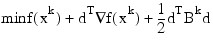
subject to:
ajd = 0, j ∈ Ik
ajd ≤ 0, j ∈ Jk
is solved to get (dk, λk) where aj is a row vector representing either a constraint in A1 or A2 or a bound constraint on x. In the latter case, the aj = ei for the bound constraint xi ≤ (xu)i and aj = -ei for the constraint -xi ≤ (xl)i. Here, ei is a vector with 1 as the i-th component, and zeros elsewhere. Variables λk are the Lagrange multipliers, and Bk is a positive definite approximation to the second derivative ∇2 f(xk).
After the search direction dk is obtained, a line search is performed to locate a better point. The new point xk+1 = xk +αkdk has to satisfy the conditions:
f(xk + αkdk) ≤ f(xk) + 0.1 * αk(dk)T ∇ f(xk)
and:
(dK)T∇ f(xk + αkdk) ≤ 0.7 * (dk)T∇ f(xK)
The main idea in forming the set Jk is that, if any of the equality constraints restricts the step-length αk, then its index is not in Jk. Therefore, small steps are likely to be avoided.
Finally, the second derivative approximation BK, is updated by the BFGS formula, if the condition:
(dK)T∇ f(xk + αkdk) − ∇ f(xk) > 0
holds. Let xk ← xk+1, and start another iteration. The iteration repeats until the stopping criterion:
|| ∇ f(xk) - AkλK||2 ≤ τ
is satisfied. Here, τ is the supplied tolerance. For more details, see Powell (1988, 1989).
Since a finite difference method is used to approximate the gradient for some single precision calculations, an inaccurate estimate of the gradient may cause the algorithm to terminate at a noncritical point. In such cases, high precision arithmetic is recommended. Also, if the gradient can be easily provided, the input keyword GRAD should be used.
Examples
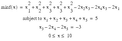
Example 1
In this example, the problem:
.RUN
FUNCTION fcn, x
f = x(0)*x(0) + x(1)*x(1) + x(2)*x(2) + x(3)*x(3) + $
x(4)*x(4) - 2.0*x(1)*x(2) - 2.0*x(3) * x(4) - $
2.0*x(0) RETURN, f
END
meq = 2
a = TRANSPOSE([[1.0, 1.0, 1.0, 1.0, 1.0], $
[0.0, 0.0, 1.0, -2.0, -2.0]])
b = [5.0, -3.0]
xlb = FLTARR(5)
xlb(*) = 0.0
xub = FLTARR(5)
xub(*) = 10.0
!QUIET = 1
x = IMSL_MINCONGEN('fcn', a, b, xlb, xub, Meq = meq)
PM, x, Title = 'Solution'
IDL prints:
Solution
1.00000
1.00000
1.00000
1.00000
1.00000
Example 2
In this example, the problem from Schittkowski (1987):
min f(x) = -x0x1x2
subject to –x0 – 2x1 – 2x2 ≤ 0 x0 + 2x1 + 2x2 ≤ 72
0 ≤ x0 ≤ 20
0 ≤ x1 ≤ 11
0 ≤ x2 ≤ 42
is solved with an initial guess of x0 = 10, x1 = 10 and x2 = 10.
.RUN
FUNCTION fcn, x
f = -x(0)*x(1)*x(2) RETURN, f
END
.RUN
FUNCTION gradient, x
g = FLTARR(3)
g(0) = -x(1)*x(2)
g(1) = -x(0)*x(2)
g(2) = -x(0)*x(1)
RETURN, g
END
meq = 0
a = TRANSPOSE([[-1.0, -2.0, -2.0], [1.0, 2.0, 2.0]])
b = [0.0, 72.0]
xlb = FLTARR(3)
xlb(*) = 0.0
xub = [20.0, 11.0, 15.0]
xguess = FLTARR(3)
xguess(*) = 10.0
!QUIET = 1
x = IMSL_MINCONGEN('fcn', a, b, xlb, xub, Meq = meq, $
Grad = 'gradient', Xguess = xguess, Obj = obj)
PM, x, Title = 'Solution'
IDL prints:
Solution
20.0000
11.0000
15.0000
Continue:
PRINT, 'Objective value =', obj
IDL prints:
Objective value = -3300.00
Syntax
Result = IMSL_MINCONGEN(f, A, B, xlb, xub [, ACTIVE_CONST=variable] [, /DOUBLE] [, GRAD=string] [, LAGRANGE_MULT=variable] [, MAX_FCN=value] [, MEQ=value] [, NUM_ACTIVE=variable] [, OBJ=variable] [, TOLERANCE=value] [, XGUESS=array])
Return Value
One-dimensional array of length nvar containing the computed solution.
Arguments
a
Two-dimensional array of size ncon by nvar containing the equality constraint gradients in the first MEQ rows followed by the inequality constraint gradients, where ncon is the number of linear constraints (excluding simple bounds) and nvar is the number of variables. See the keyword MEQ for setting the number of equality constraints.
b
One-dimensional array of size ncon containing the right-hand sides of the linear constraints. Specifically, the constraints on the variables xi, i = 0, nvar – 1, are ak,0x0 + ... + ak,nvar–1xnvar–1 = bk, k = 0, ..., MEQ – 1 and ak,0x0 + ... + ak,nvar–1xnvar–1 ≤ bk, k = MEQ, ..., ncon – 1. Note that the data that define the equality constraints come before the data of the inequalities.
f
Scalar string specifying a user-supplied function to evaluate the function to be minimized. Function f accepts a one-dimensional array of length n = N_ELEMENTS(x) containing the point at which the function is evaluated. The return value of this function is the function value at x.
xlb
One-dimensional array of length nvar containing the lower bounds on the variables; choose a very large negative value if a component should be unbounded below, or set xlb(i) = xub(i) to freeze the i-th variable. Specifically, these simple bounds are xlb(i) ≤ xi, for i = 0, ..., nvar–1.
xub
One-dimensional array of length nvar containing the upper bounds on the variables; choose a very large positive value if a component should be unbounded above. Specifically, these simple bounds are xi ≤ xub(i), for i = 0, nvar – 1.
Keywords
ACTIVE_CONST (optional)
Named variable in the form of a one-dimensional array of length NUM_ACTIVE containing the indices of the final active constraints.
DOUBLE (optional)
If present and nonzero, then double precision is used.
GRAD (optional)
Scalar string specifying the name of the user-supplied function to compute the gradient at the point x. The GRAD function accepts a one-dimensional array of length nvar. The return value of this function is a one-dimensional array of length nvar containing the values of the gradient of the objective function.
LAGRANGE_MULT (optional)
Named variable in the form of a one-dimensional array of length NUM_ACTIVE containing the Lagrange multiplier estimates of the final active constraints.
MAX_FCN (optional)
Maximum number of function evaluations. The default value is 400.
MEQ (optional)
Number of linear equality constraints. The default value is 0.
NUM_ACTIVE (optional)
Named variable containing the final number of active constraints.
OBJ (optional)
Named variable containing the value of the objective function.
TOLERANCE (optional)
The nonnegative tolerance on the first order conditions at the calculated solution. The default value is SQRT(ε), where ε is machine epsilon.
XGUESS (optional)
One-dimensional array with nvar components containing an initial guess. The default value is 0.
Version History