The IMSL_NLINLSQ function solves a nonlinear least-squares problem using a modified Levenberg-Marquardt algorithm.
This routine requires an IDL Advanced Math and Stats license. For more information, contact your sales or technical support representative.
The specific algorithm used in IMSL_NLINLSQ is dependent on whether the keywords XLB and XUB are supplied. If the keywords XLB and XUB are not supplied, then the IMSL_NLINLSQ function is based on the MINPACK routine LMDER by Moré et al. (1980).
The IMSL_NLINLSQ function, based on the MINPACK routine LMDER by Moré et al. (1980), uses a modified Levenberg-Marquardt method to solve nonlinear least- squares problems. The problem is stated as follows:
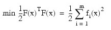
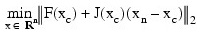
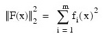
where m ≥ n, F : Rn → Rm and fi (x) is the i-th component function of F(x). From a current point, the algorithm uses the trust region approach:
subject to 
to get a new point xn. Compute xn as:
xn = xc – (J(xc)T J(xcμ) + mc I )–1 J(xc)TF(xc)
where μc = 0 if dc ³ || (J(xc)T J(xc))–1 J(xc)TF(xc) ||2 and μc > 0 otherwise.
The value μc is defined by the function. The vector and matrix F(xc) and J(xc) are the function values and the Jacobian evaluated at the current point xc. This function is repeated until the stopping criteria are satisfied.
The first stopping criterion for IMSL_NLINLSQ occurs when the norm of the function is less than the absolute function tolerance, TOL_AFCN. The second stopping criterion occurs when the norm of the scaled gradient is less than the given gradient tolerance TOL_GRAD. The third stopping criterion for IMSL_NLINLSQ occurs when the scaled distance between the last two steps is less than the step tolerance TOL_STEP. For more details, see Levenberg (1944), Marquardt (1963), or Dennis and Schnabel (1983, Chapter 10).
If the keywords XLB and XUB are supplied, then the IMSL_NLINLSQ function uses a modified Levenberg-Marquardt method and an active set strategy to solve nonlinear least-squares problems subject to simple bounds on the variables. The problem is stated as follows:
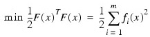
subject to l ≤ x ≤ u where m ≥ n, F : Rn → Rm, and fi(x) is the i-th component function of F(x). From a given starting point, an active set IA, which contains the indices of the variables at their bounds, is built. A variable is called a “free variable” if it is not
in the active set. The routine then computes the search direction for the free variables according to the formula:
d = – (JTJ + µI)–1 JTF
where µ is the Levenberg-Marquardt parameter, F = F(x), and J is the Jacobian with respect to the free variables. The search direction for the variables in IA is set to zero. The trust region approach discussed by Dennis and Schnabel (1983) is used to find the new point. Finally, the optimality conditions are checked. The conditions are:
||g (xi)|| ≤ ε, li < xi < ui
g (xi) < 0, xi = ui
g (xi) > 0, xi = li
where ε is a gradient tolerance. This process is repeated until the optimality criterion is achieved.
The active set is changed only when a free variable hits its bounds during an iteration or the optimality condition is met for free variables but not for all variables in IA, the active set. In the latter case, a variable that violates the optimality condition will be dropped out of IA. For more detail on the Levenberg-Marquardt method, see Levenberg (1944) or Marquardt (1963). For more detail on the active set strategy, see Gill and Murray (1976).
Since a finite-difference method is used to estimate the Jacobian for some single- precision calculations, an inaccurate estimate of the Jacobian may cause the algorithm to terminate at a noncritical point. In such cases, high-precision arithmetic is recommended. Also, whenever the exact Jacobian can be easily provided, the keyword JACOBIAN should be used.
Example
In this example, the nonlinear data-fitting problem found in Dennis and Schnabel (1983, p. 225):
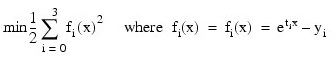
is solved with the data t = [1, 2, 3] and y = [2, 4, 3].
.RUN
FUNCTION f, m, x
y = [2, 4, 3]
t = [1, 2, 3]
RETURN, EXP(x(0) * t) - y
END
solution = IMSL_NLINLSQ('f', 3, 1)
PM, solution, Title = 'The solution is:'
IDL prints:
The solution is:
0.440066
PM, f(m, solution), Title = 'The function values are:'
IDL prints:
The function values are:
-0.447191
-1.58878
0.744159
Errors
Informational Errors
MATH_STEP_TOLERANCE: Scaled step tolerance satisfied. The current point may be an approximate local solution, but it is also possible that the algorithm is making very slow progress and is not near a solution or that TOL_STEP is too big.
Warning Errors
MATH_LITTLE_FCN_CHANGE: Both the actual and predicted relative reductions in the function are less than or equal to the relative function tolerance.
MATH_TOO_MANY_ITN: Maximum number of iterations exceeded.
MATH_TOO_MANY_FCN_EVAL: Maximum number of function evaluations exceeded.
MATH_TOO_MANY_JACOBIAN_EVAL: Maximum number of Jacobian evaluations exceeded.
MATH_UNBOUNDED: Five consecutive steps have been taken with the maximum step length.
Fatal Errors
MATH_FALSE_CONVERGE: Iterates appear to be converging to a noncritical point.
Syntax
Result = IMSL_NLINLSQ(F, M, N [, Xlb] [, Xub] [, /DOUBLE] [, FJAC=variable] [, FSCALE=array] [, FVEC=variable] [, INTERN_SCALE=variable] [, ITMAX=value] [, JACOBIAN=string] [, JTJ_INVERSE=variable] [, MAX_EVALS=value] [, MAX_JACOBIAN=value] [, MAX_STEP=value] [, N_DIGITS=value] [, RANK=value] [, TOL_AFCN=value] [, TOL_GRAD=value] [, TOL_RFCN=value] [, TOL_STEP=value] [, TOLERANCE=value] [, TRUST_REGION=value] [, XGUESS=array] [, XSCALE=array])
Return Value
The solution x of the nonlinear least-squares problem. If no solution can be computed, NULL is returned.
Arguments
F
Scalar string specifying a user-supplied function to evaluate the function that defines the least-squares problem. The argument F accepts the following two parameters and returns an array of length m containing the function values at x:
- m: Number of functions.
- x: Array length n containing the point at which the function is evaluated.
M
Number of functions.
N
Number of variables where n ≤ m.
Xlb
One dimensional array with n components containing the lower bounds on the variables. The Xlb and Xub arguments must be used together.
Xub
One dimensional array with n components containing the upper bounds on the variables. The Xlb and Xub arguments must be used together.
Keywords
DOUBLE (optional)
If present and nonzero, then double precision is used.
FJAC (optional)
Name of the variable into which an array of size m x n containing the Jacobian at the approximate solution is stored.
FSCALE (optional)
Array with m components containing the diagonal scaling matrix for the functions. The i-th component of FSCALE is a positive scalar specifying the reciprocal magnitude of the i-th component function of the problem. Default: FSCALE (*) = 1.
FVEC (optional)
Name of the variable into which a real array of length m containing the residuals at the approximate solution is stored.
INTERN_SCALE (optional)
Internal variable scaling option. With this keyword, the values for XSCALE are set internally.
ITMAX (optional)
Maximum number of iterations. Default: 100.
JACOBIAN (optional)
Scalar string specifying a user-supplied function to compute the Jacobian. This function accepts two parameters and returns an n x m array containing the Jacobian at the point s input point. Note that each derivative ∂fi/∂xj should be returned in the (i, j) element of the returned matrix. The parameters of the function are as follows:
- m: Number of equations.
- x: Array of length n at which the point Jacobian is evaluated.
JTJ_INVERSE (optional)
Name of the variable into which an array of size n x n containing the inverse matrix of JTJ, where J is the final Jacobian, is stored. If JTJ is singular, the inverse is a symmetric g2 inverse of JTJ. (See IMSL_CHNNDSOL for a discussion of generalized inverses and the definition of the g2 inverse.)
MAX_EVALS (optional)
Maximum number of function evaluations. Default: 400.
MAX_JACOBIAN (optional)
Maximum number of Jacobian evaluations. Default: 400.
MAX_STEP (optional)
Maximum allowable step size. Default: 1000 max(ε1, ε2), where:
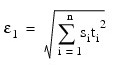

s = XSCALE, and t = XGUESS
N_DIGITS (optional)
Number of good digits in the function. Default: machine dependent.
RANK (optional)
Name of the variable into which the rank of the Jacobian is stored.
TOL_AFCN (optional)
Absolute function tolerance. Default: max(10–20, ε2), [max(10–40, ε2) in double], where ε is the machine precision.
TOL_GRAD (optional)
Scaled gradient tolerance.
The i-th component of the scaled gradient at x is calculated as:
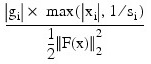
where g = ∇F(x) , s = XSCALE, and:
Default: ε1/2 (ε1/3 in double), where ε is the machine precision.
TOL_RFCN (optional)
Relative function tolerance. Default: max(10–10, ε2/3), [max(10–40, ε2/3) in double], where ε is the machine precision.
TOL_STEP (optional)
Scaled step tolerance.
The i-th component of the scaled step between two points x and y is computed as:
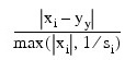
where s = XSCALE.
Default: ε2/3, where ε is the machine precision
TOLERANCE (optional)
Tolerance used in determining linear dependence for the computation of the inverse of JTJ. If the keyword JACOBIAN is specified, the default is 100ε, where ε is the machine precision; otherwise, the default is SQRT(ε), where ε is the machine precision.
TRUST_REGION (optional)
Size of initial trust-region radius. Default: based on the initial scaled Cauchy step.
XGUESS (optional)
Array with n components containing an initial guess. Default: XGUESS (*) = 0.
XSCALE (optional)
Array with n components containing the scaling vector for the variables. The keyword XSCALE is used mainly in scaling the gradient and the distance between two points (see the keywords TOL_GRAD and TOL_STEP for more detail). Default: XSCALE (*) = 1.
Version History
See Also
IMSL_CHNNDSOL