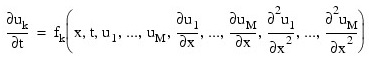
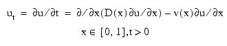
The IMSL_PDE_MOL function solves a system of partial differential equations of the form ut = f(x, t, u, ux, uxx) using the method of lines. The solution is represented with cubic Hermite polynomials.
This routine requires an IDL Advanced Math and Stats license. For more information, contact your sales or technical support representative.
Let M = npde, N = nx and xi = xbreak(i). The routine IMSL_PDE_MOL uses the method of lines to solve the partial differential equation system:
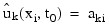
with the initial conditions:
uk = uk(x, t) at t = t0, where t0 = t(0)
and the boundary conditions:

for k = 1, ..., M.
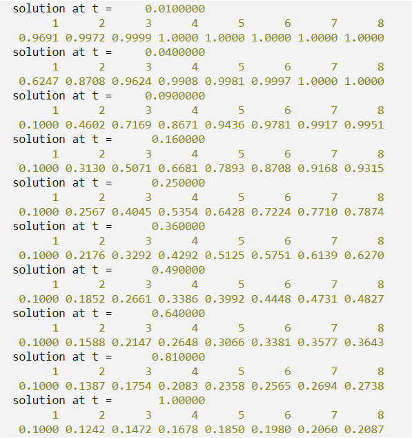
Cubic Hermite polynomials are used in the x variable approximation so that the trial solution is expanded in the series:
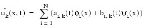
where φi(x) and ψi(x) are standard basis functions for cubic Hermite polynomials with the knots x1 < x2 < ... < xN. These are piecewise cubic polynomials with continuous first derivatives. At the breakpoints, they satisfy:

According to the collocation method, the coefficients of the approximation are obtained so that the trial solution satisfies the differential equation at the two Gaussian points in each subinterval:
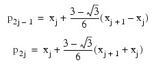
for j = 1, ..., N. The collocation approximation to the differential equation is:

for k = 1, ..., M and j = 1, ..., 2(N − 1).
This is a system of 2M(N - 1) ordinary differential equations in 2M N unknown coefficient functions, ai,k and bi,k. This system can be written in the matrix-vector form as A dc/dt = F (t, y) with c(t0) = c0 where c is a vector of coefficients of length 2M N and c0 holds the initial values of the coefficients. The last 2M equations are obtained by differentiating the boundary conditions:
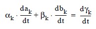
for k = 1, ..., M.
The initial conditions uk(x, t0) must satisfy the boundary conditions. Also, the gk(t) must be continuous and have a smooth derivative, or the boundary conditions will not be properly imposed for t > t0.
If ak = bk = 0, it is assumed that no boundary condition is desired for the k-th unknown at the left endpoint. A similar comment holds for the right endpoint. Thus, collocation is done at the endpoint. This is generally a useful feature for systems of first-order partial differential equations.
If the number of partial differential equations is M = 1 and the number of breakpoints is N = 4, then:
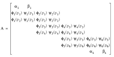
The vector c is:
c = [a1, b1, a2, b2, a3, b3, a4, b4]T
and the right-side F is:

If M > 1, then each entry in the above matrix is replaced by an M x M diagonal matrix. The element a1 is replaced by diag(a1,1, ..., a1,M ). The elements aN, β1 and βN are handled in the same manner. The fi(pj) and yi(pj) elements are replaced by fi(pj)IM and yi(pj)IM where IM is the identity matrix of order M. See Madsen and Sincovec (1979) for further details about discretization errors and Jacobian matrix structure.
The input array y contains the values of the ak,i. The initial values of the bk,i are obtained by using the cubic spline routine IMSL_CSINTERP to construct functions:

such that:
The IDL Advanced Math and Stats routine IMSL_SPVALUE is used to approximate the values:
There is an optional use of IMSL_PDE_MOL that allows the user to provide the initial values of bk,i.
The order of matrix A is 2MN and its maximum bandwidth is 6M − 1. The band structure of the Jacobian of F with respect to c is the same as the band structure of A. This system is solved using a modified version of IMSL_ODE. Some of the linear solvers were removed. Numerical Jacobians are used exclusively. The algorithm is unchanged. Gear’s BDF method is used as the default because the system is typically stiff.
Four examples of PDEs are now presented that illustrate how users can interface their problems with IMSL_PDE_MOL. The examples are small and not indicative of the complexities that most practitioners will face in their applications.
Examples
Example 1
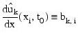
This equation solves the normalized linear diffusion PDE, ut = uxx, 0 ≤ x ≤ 1, t > t0. The initial values are t0 = 0, u(x, t0) = u0 = 1. There is a "zero-flux" boundary condition at x = 1, namely ux(1, t) = 0, (t > t0). The boundary value of u(0, t) is abruptly changed from u0 to the value u1 = 0.1. This transition is completed by t = td = 0.09.
Due to restrictions in the type of boundary conditions successfully processed by IMSL_PDE_MOL, it is necessary to provide the derivative boundary value function g¢ at x = 0 and at x = 1. The function g at x = 0 makes a smooth transition from the value u0 at t = t0 to the value u1 at t = td. The transition phase for g¢ is computed by evaluating a cubic interpolating polynomial. For this purpose, the function subprogram IMSL_SPVALUE. The interpolation is performed as a first step in the user-supplied procedure f_bc. The function and derivative values g(t0) = u0, g¢(t0) = 0, g(td) = u1, and g¢(td) = 0, are used as input to routine IMSL_CSINTERP to obtain the coefficients evaluated by IMSL_SPVALUE. Notice that g¢(t) = 0, t > td. The evaluation routine IMSL_SPVALUE will not yield this value so logic in the procedure f_bc assigns g¢(t) = 0, t > td.
Save the following code as pde_mol_example1, then compile and run:
FUNCTION f_ut, npde, x, t, u, ux, uxx
ut = uxx RETURN, ut
END
PRO f_bc, npde, x, t, alpha, beta, gammap
COMMON ex1_pde, first, ppoly first = 1
alpha = FLTARR(npde) beta = FLTARR(npde)
gammap = FLTARR(npde) delta = 0.09
IF (first EQ 1) THEN BEGIN
first = 0
ppoly = IMSL_CSINTERP([0.0, delta], [1.0, 0.1], $
ileft = 1, left = 0.0, iright = 1, right = 0.0)
ENDIF
IF (x EQ 0.0) THEN BEGIN
alpha(0) = 1.0
beta(0) = 0.0
gammap(0) = 0.0
IF (t LE delta) THEN gammap(0) = $
IMSL_SPVALUE(t, ppoly, xderiv = 1)
END ELSE BEGIN
alpha(0) = 0.0
beta(0) = 1.0
gammap(0) = 0.0
END
RETURN
END
PRO pde_mol_example1
COMMON ex1_pde, first, ppoly
npde = 1
nx = 8 nstep = 10
xbreak = FINDGEN(nx)/(nx - 1)
y = FLTARR(npde, nx)
y(*) = 1.0
t = FINDGEN(nstep)/(nstep) + 0.1
t = [0.0, t*t]
res = IMSL_PDE_MOL(t, y, xbreak, 'f_ut', 'f_bc')
num = INDGEN(8) + 1
FOR i = 1, 10 DO BEGIN
PRINT, 'solution at t = ', t(i)
PRINT, num, FORMAT = '(8I7)'
PM, res(0, *, i), FORMAT = '(8F7.4)'
ENDFOR
END
IDL Prints:
Example 2
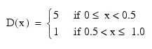
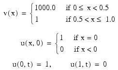
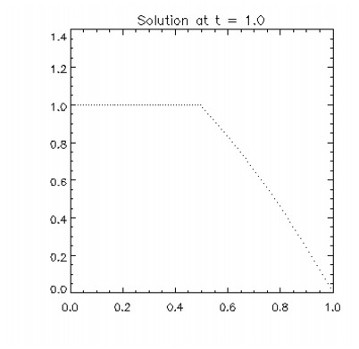
This example solves Problem C from Sincovec and Madsen (1975). The equation is of diffusion-convection type with discontinuous coefficients. This problem illustrates a simple method for programming the evaluation routine for the derivative, ut. Note that the weak discontinuities at x = 0.5 are not evaluated in the expression for ut. The results are shown in the figure that follows. The problem is defined as:
Save the following code as pde_mol_example2, then compile and run:
FUNCTION f_ut, npde, x, t, u, ux, uxx
ut = FLTARR(npde)
IF (x LE 0.5) THEN BEGIN
d = 5.0
v = 1000.0
END ELSE BEGIN
d = 1.0
v = 1.0
END
ut(0) = d*uxx(0) - v*ux(0)
RETURN, ut
END
PRO f_bc, npde, x, t, alpha, beta, gammap
alpha = FLTARR(npde)
beta = FLTARR(npde)
gammap = FLTARR(npde) alpha(0) = 1.0
beta(0) = 0.0
gammap(0) = 0.0
RETURN
END
PRO pde_mol_example2
npde = 1
nx = 100 nstep = 10
xbreak = FINDGEN(nx)/(nx - 1)
y = FLTARR(npde, 100)
y(*) = 0.0 y(0) = 1.0
mach = IMSL_MACHINE(/FLOAT)
tol = SQRT(mach.MAX_REL_SPACE)
hinit = 0.01*tol
PRINT, 'tol = ', tol, ' and hinit = ', hinit
t = [0.0, FINDGEN(nstep)/(nstep) + 0.1]
res = IMSL_PDE_MOL(t, y, xbreak, 'f_ut', 'f_bc', $
tolerance = tol, hinit = hinit)
PLOT, xbreak, res(0,*,10), psym = 3, yrange=[0 , 1.25], $
title = 'Solution at t = 1.0'
END
Example 3
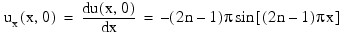
n this example, using IMSL_PDE_MOL, the linear normalized diffusion PDE ut = uxx is solved but with an optional use that provides values of the derivatives, ux, of the initial data. Due to errors in the numerical derivatives computed by spline interpolation, more precise derivative values are required when the initial data is u(x, 0) = 1 + cos[(2n - 1)πx], n > 1. The boundary conditions are "zero flux" conditions ux(0, t) = ux(1, t) = 0 for t > 0. Note that the initial data is compatible with these end conditions since the derivative function:
vanishes at x = 0 and x = 1.
This optional usage signals that the derivative of the initial data is passed by the user.
Save the following code as pde_mol_example3, then compile and run:
FUNCTION f_ut, npde, x, t, u, ux, uxx
ut = fltARR(npde)
ut(0) = uxx(0) RETURN, ut
END
PRO f_bc, npde, x, t, alpha, beta, gammap
alpha = FLTARR(npde)
beta = FLTARR(npde)
gammap = FLTARR(npde)
alpha(0) = 0.0
beta(0) = 1.0
gammap(0) = 0.0
RETURN
END
PRO pde_mol_example3
npde = 1
nx = 10 nstep = 10
arg = 9.0*!Pi
xbreak = FINDGEN(nx)/(nx - 1)
y = FLTARR(npde, nx)
y(0, *) = 1.0 + COS(arg*xbreak)
di = y
di(0, *) = -arg*SIN(arg*xbreak)
mach = IMSL_MACHINE(/FLOAT)
tol = SQRT(mach.MAX_REL_SPACE)
t = [FINDGEN(nstep + 1)*(nstep*0.001)/(nstep)]
res = IMSL_PDE_MOL(t, y, xbreak, 'f_ut', 'f_bc', $
Tolerance = tol, Deriv_Init = di)
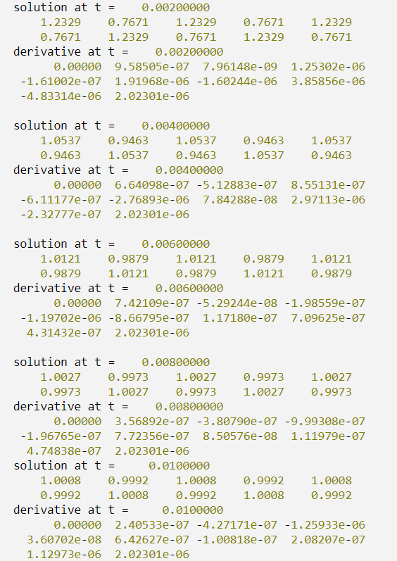
FOR i = 2, 10, 2 DO BEGIN
PRINT, 'solution at t = ', t(i)
PM, res(0, *, i), FORMAT = '(10F10.4)'
PRINT, 'derivative at t = ', t(i)
PM, di(0, *, i)
PRINT
ENDFOR
END
IDL Prints:
Example 4
In this example, consider the linear normalized hyperbolic PDE, utt = uxx, the "vibrating string" equation. This naturally leads to a system of first order PDEs. Define a new dependent variable ut = v. Then, vt = uxx is the second equation in the system. Take as initial data u(x, 0) = sin(πx) and ut(x, 0) = v(x, 0) = 0. The ends of the string are fixed so u(0, t) = u(1, t) = v(0, t) = v(1, t) = 0. The exact solution to this problem is u(x, t) = sin(πx) cos(πt). Residuals are computed at the output values of t for 0 < t ≤ 2. Output is obtained at 200 steps in increments of 0.01.
Even though the sample code IMSL_PDE_MOL gives satisfactory results for this PDE, be aware that for nonlinear problems, “shocks” can develop in the solution. The appearance of shocks may cause the code to fail in unpredictable ways. See Courant and Hilbert (1962), pp 488-490, for an introductory discussion of shocks in hyperbolic systems.
Save the following code as pde_mol_example4, then compile and run:
FUNCTION f_ut, npde, x, t, u, ux, uxx
ut = FLTARR(npde)
ut(0) = u(1)
ut(1) = uxx(0)
RETURN, ut
END
PRO f_bc, npde, x, t, alpha, beta, gammap
alpha = FLTARR(npde)
beta = FLTARR(npde)
gammap = FLTARR(npde)
alpha(0) = 1
alpha(1) = 1
beta(0) = 0
beta(1) = 0
gammap(0) = 0
gammap(1) = 0
RETURN
END
PRO pde_mol_example4
npde = 2
nx = 10
nstep = 200
xbreak = FINDGEN(nx)/(nx - 1)
y = FLTARR(npde, nx)
y(0, *) = SIN(!Pi*xbreak)
y(1, *) = 0 di = y
di(0, *) = !Pi*COS(!Pi*xbreak)
di(1, *) = 0.0
mach = IMSL_MACHINE(/FLOAT)
tol = SQRT(mach.MAX_REL_SPACE)
t = [0.0, 0.01 + FINDGEN(nstep)*2.0/(nstep)]
u = IMSL_PDE_MOL(t, y, xbreak, 'f_ut', 'f_bc', $
Tolerance = tol, Deriv_Init = di)
err = 0.0
pde_error = FLTARR(nstep)
FOR j = 1, N_ELEMENTS(t) - 1 DO BEGIN
FOR i = 0, nx - 1 DO BEGIN
err = (err) > (u(0, i, j) - $
SIN(!Pi*xbreak(i))*COS(!Pi*t(j)))
ENDFOR
ENDFOR
PRINT, 'Maximum error in u(x, t) = ', err
END
IDL Prints:
Maximum error in u(x, t) = 0.000626385
Syntax
Result = IMSL_PDE_MOL(T, Y, Xbreak, F_Ut, F_Bc, Gammap [, /DOUBLE] [, DERIV_INIT=array] [, HINIT=value] [, TOLERANCE=value])
Return Value
Three-dimensional array of size npde by nx by N_ELEMENTS(t) containing the approximate solutions for each specified value of the independent variable.
Arguments
T
One-dimensional array containing values of independent variable. Element t(0) should contain the initial independent variable value (the initial time, t0) and the remaining elements of t should be values of the independent variable at which a solution is desired.
Y
Two-dimensional array of size npde by nx containing the initial values, where npde is the number of differential equations and nx is the number of mesh points or lines. It must satisfy the boundary conditions.
Xbreak
One-dimensional array of length nx containing the breakpoints for the cubic Hermite splines used in the x discretization. The points in xbreak must be strictly increasing. The values Xbreak(0) and Xbreak(nx − 1) are the endpoints of the interval.
F_Ut
Scalar string specifying an user-supplied function to evaluate ut. Function f_ut accepts the following arguments:
- npde: Number of equations.
- x: Space variable, x.
- t: Time variable, t.
- u: One-dimensional array of length npde containing the dependent values, u.
- ux: One-dimensional array of length npde containing the first derivatives, ux.
- uxx: One-dimensional array of length npde containing the second derivative, uxx.
The return value of this function is an one-dimensional array of length npde containing the computed derivatives ut.
F_Bc
Scalar string specifying user-supplied procedure to evaluate boundary conditions. The boundary conditions accepted by IMSL_PDE_MOL are:
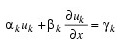
Note: You must supply the values αk and βk, which determine the values γk. Since γk can depend on t values, γk' also are required.
- npde: Number of equations. (Input)
- x: Space variable, x. (Input)
- t: Time variable, t. (Input)
- alpha: Named variable into which an one-dimensional array of length npde containing the αk values is stored. (Output)
- beta Named variable into which an one-dimensional array of length npde containing the βk values is stored. (Output)
Gammap
Named variable into which an one-dimensional array of length npde containing the derivatives is stored. (Output):

Keywords
DOUBLE (optional)
If present and nonzero, then double precision is used.
DERIV_INIT (optional)
Two-dimensional array that supplies the derivative values ux(x, t(0)). This derivative information is input as:
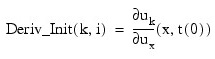
Default: Derivatives are computed using cubic spline interpolation
HINIT (optional)
Initial step size in the t integration. This value must be nonnegative. If HINIT is zero, an initial step size of 0.001|ti+1 - ti| will be arbitrarily used. The step will be applied in the direction of integration. Default: 0.0
TOLERANCE (optional)
Differential equation error tolerance. An attempt to control the local error in such a way that the global relative error is proportional to TOLERANCE. Default: 100.0*ε, where ε is machine epsilon.
Version History
See Also
IMSL_CSINTERP, IMSL_SPVALUE