The IMSL_POLYPREDICT function computes predicted values, confidence intervals, and diagnostics after fitting a polynomial regression model.
This routine requires an IDL Advanced Math and Stats license. For more information, contact your sales or technical support representative.
The IMSL_POLYPREDICT function assumes a polynomial model
yi = β 0 + β 1xi + ..., β kxki + εi i = 1, 2, ..., n
where the observed values of the yi’s constitute the response, the xi’s are the settings of the independent variable, the βj’s are the regression coefficients, and the εi’s are the errors that are independently distributed normal with mean zero and the following variance:
σ2/wi
Given the results of a polynomial regression, fitted using orthogonal polynomials and weights wi, IMSL_POLYPREDICT produces predicted values, residuals, confidence intervals, prediction intervals, and diagnostics for outliers and in influential cases.
Often, a predicted value and confidence interval are desired for a setting of the independent variable not used in computing the regression fit. This is accomplished by simply using a different x matrix than was used for the fit when calling IMSL_POLYPREDICT (IMSL_POLYREGRESS).
Results from IMSL_POLYREGRESS, which produces the fit using orthogonal polynomials, are used for input by the array predict_info. The fitted model from IMSL_POLYREGRESS is:
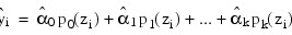
where the zi’s are settings of the independent variable x scaled to the interval [–2, 2] and the pj (z)’s are the orthogonal polynomials. The XTX matrix for this model is a diagonal matrix with elements dj. The case statistics are easily computed from this model and are equal to those from the original polynomial model with βj’s as the regression coefficients.
The leverage is computed as follows:
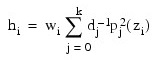
The estimated variance of:


The computation of the remainder of the case statistics follow easily from their definitions. See the IMSL introduction for the definition of the case diagnostics.
Often, predicted values and confidence intervals are desired for combinations of settings of the independent variables not used in computing the regression fit. This can be accomplished by defining a new data matrix. Since the information about the model fit is input in predict_info, it is not necessary to send in the data set used for the original calculation of the fit, i.e., only variable combinations for which predictions are desired need be entered in x.
Examples
Example 1
A polynomial model is fit to data using the IMSL_POLYREGRESS routine, then IMSL_POLYPREDICT is used to compute predicted values. The results are shown in the figure that follows.
x = [0, 0, 1, 1, 2, 2, 4, 4, 5, 5, 6, 6, 7, 7]
y = [58, 48, 58, 57, 61, 67, 70, 74, 77, 72, 81, 85, 84, 81]
Coefs = IMSL_POLYREGRESS(x, y, degree, $
Predict_Info = predict_info)
x2 = 8 * FINDGEN((100)/99)
predicted = IMSL_POLYPREDICT(predict_info, x2)
PLOT, x, y, Psym = 4
OPLOT, x2, predicted
Example 2
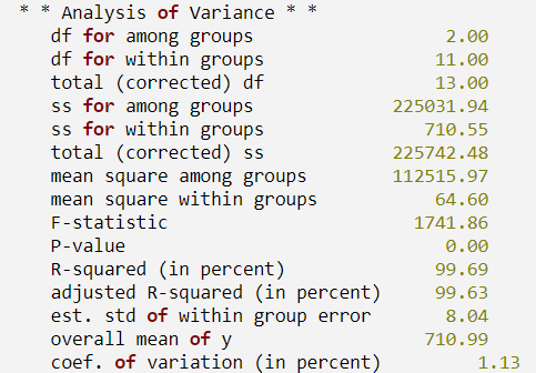
A polynomial model is fit to the data discussed by Neter and Wasserman (1974, pp. 279-285). The data set contains the response variable y measuring coffee sales (in hundreds of gallons) and the number of self-service dispensers. Responses for 14 similar cafeterias are in the data set. First, a procedure is defined to print the ANOVA table. The results are shown in the figure that follows.
.RUN
PRO print_results, anova_table
'df for within groups ', $
'total (corrected) df ', $
'ss for among groups ', $
'ss for within groups ', $
'total (corrected) ss ', $
'mean square among groups ', $
'mean square within groups ', $
'F-statistic ', $
'P-value ', $
'R-squared (in percent) ', $
'adjusted R-squared (in percent)', $
'est. std of within group error ', $
'overall mean of y ', $
'coef. of variation (in percent)']
PRINT, ' * * Analysis of Variance * *'
anova_table(i), FORMAT = '(a32,f10.2)'
END
x = [0, 0, 1, 1, 2, 2, 4, 4, 5, 5, 6, 6, 7, 7]
y = [508.1, 498.4, 568.2, 577.3, 651.7, $
657.0, 755.3, 758.9, 787.6, 792.1, $
841.4, 831.8, 854.7, 871.4]
degree = 2
coefs = IMSL_POLYREGRESS(x, y, degree, $
Anova_Table = anova_table, predict_info = predict_info)
Ci_Scheffe = ci_scheffe, Y = y, Dffits = dffits)
PLOT, x, ci_scheffe(1, *), Yrange = [450, 900], Linestyle = 2
OPLOT, x, y, Psym = 4
x2 = 7 * FINDGEN(100)/99
OPLOT, x2, IMSL_POLYPREDICT(predict_info, x2)
print_results, anova_table
Result:
Errors
Warning Errors
STAT_LEVERAGE_GT_1: Leverage (= #) much greater than 1 is computed. It is set to 1.0.
STAT_DEL_MSE_LT_0: Deleted residual mean square (= #) much less than zero is computed. It is set to zero.
Fatal Errors
STAT_NEG_WEIGHT: Keyword Weights(#) = #. Weights must be nonnegative.
Syntax
Result = IMSL_POLYPREDICT(Predict_Info, X [, CI_PTW_NEW_SAMP=variable] [, CI_PTW_POP_MEAN=variable] [, CI_SCHEFFE=variable] [, CONFIDENCE=value] [, COOKS_D=variable] [, DEL_RESIDUAL=variable] [, DFFITS=variable] [, /DOUBLE] [, LEVERAGE=variable] [, RESIDUAL=variable] [, STD_RESIDUAL=variable] [, WEIGHTS=array] [, Y=array])
Return Value
A structure containing all the information to determine the spline fit.
Arguments
Predict_Info
One-dimensional byte array containing information computed by IMSL_POLYREGRESS and returned through keyword Predict_Info. The data contained in this array is in an encrypted format and should not be altered after it is returned by IMSL_POLYREGRESS.
X
One-dimensional array containing the values of the independent variable for which calculations are to be performed.
Keywords
CI_PTW_NEW_SAMP (optional)
Named variable into which the two-dimensional array of size 2 by N_ELEMENTS(x) containing the confidence intervals for two-sided prediction intervals, corresponding to the elements of x, is stored. Element CI_PTW_NEW_SAMP(0, i) contains the i-th lower confidence limit, CI_PTW_NEW_SAMP(1, i) contains the i-th upper confidence limit.
CI_PTW_POP_MEAN (optional)
Named variable into which the two-dimensional array of size 2 by N_ELEMENTS(x) containing the confidence intervals for two-sided interval estimates of the means, corresponding to the elements of x, is stored. Element CI_PTW_POP_MEAN(0, i) contains the i-th lower confidence limit, Ci_Ptw_Pop_Mean (1, i) contains the i-th upper confidence limit.
CI_SCHEFFE (optional)
Named variable into which the two-dimensional array of size 2 by N_ELEMENTS(x) containing the Scheffé confidence intervals, corresponding to the rows of x, is stored. Element CI_SCHEFFE(0, i) contains the i-th lower confidence limit; CI_SCHEFFE(1, i) contains the i-th upper confidence limit.
CONFIDENCE (optional)
Confidence level for both two-sided interval estimates on the mean and for two-sided prediction intervals, in percent. This keyword must be in the range (0.0, 100.0). For one-sided intervals with confidence level, where 50.0 ≤ c < 100.0, set Confidence = 100.0 – 2.0 * (100.0 – c). Default: 95.0
COOKS_D (optional)
Named variable into which the one-dimensional array of length N_ELEMENTS(x) containing the Cook’s D statistics is stored. You must specify Y when using this keyword.
DEL_RESIDUAL (optional)
Named variable into which the one-dimensional array of length N_ELEMENTS(x) containing the deleted residuals is stored. You must specify Y when using this keyword.
DFFITS (optional)
Named variable into which the one-dimensional array of length N_ELEMENTS(x) containing the DFFITS statistics is stored. You must specify Y when using this keyword.
DOUBLE (optional)
If present and nonzero, double precision is used.
LEVERAGE (optional)
Named variable into which the one-dimensional array of length N_ELEMENTS(x) containing the leverages is stored.
RESIDUAL (optional)
Named variable into which the one-dimensional array of length N_ELEMENTS(x) containing the residuals is stored. You must specify Y when using this keyword
STD_RESIDUAL (optional)
Named variable into which the one-dimensional array of length N_ELEMENTS(x) containing the standardized residuals is stored. You must specify Y when using this keyword
WEIGHTS (optional)
One-dimensional array containing the weight for each element of x. The computed prediction interval uses SSE/(DFE * Weights (i)) for the estimated variance of a future response. Default: Weights (*) = 1
Y (optional)
Array of length N_ELEMENTS (x) containing the observed responses.
Version History
See Also
IMSL_POLYREGRESS