The IMSL_POLYREGRESS function performs a polynomial least-squares regression.
This routine requires an IDL Advanced Math and Stats license. For more information, contact your sales or technical support representative.
The IMSL_POLYREGRESS function computes estimates of the regression coefficients in a polynomial (curvilinear) regression model. In addition to the computation of the fit, IMSL_POLYREGRESS computes some summary statistics. Sequential sum of squares attributable to each power of the independent variable (returned by using Ssq_Poly) are computed. These are useful in assessing the importance of the higher order powers in the fit. Draper and Smith (1981, pp. 101–102) and Neter and Wasserman (1974, pp. 278–287) discuss the interpretation of the sequential sum of squares.
The statistic R2 is the percentage of the sum of squares of y about its mean explained by the polynomial curve. Specifically:
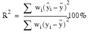
where wi is the weight.

is the fitted y value at xi and

is the mean of y. This statistic is useful in assessing the overall fit of the curve to the data. R2 must be between 0% and 100%, inclusive. R2 = 100% indicates a perfect fit to the data.
Estimates of the regression coefficients in a polynomial model are computed using orthogonal polynomials as the regressor variables. This reparameterization of the polynomial model in terms of orthogonal polynomials has the advantage that the loss of accuracy resulting from forming powers of the x-values is avoided. All results are returned to you for the original model (power form).
The IMSL_POLYREGRESS function is based on the algorithm of Forsythe (1957). A modification to Forsythe’s algorithm suggested by Shampine (1975) is used for computing the polynomial coefficients. A discussion of Forsythe’s algorithm and Shampine’s modification appears in Kennedy and Gentle (1980, pp. 342–347).
Examples
Example 1
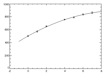
A polynomial model is fitted to data discussed by Neter and Wasserman (1974, pp. 279–285). The data set contains the response variable y measuring coffee sales (in hundred gallons) and the number of self-service coffee dispensers. Responses for fourteen similar cafeterias are in the data set. The results are shown the figure that follows.
x = [0, 0, 1, 1, 2, 2, 4, 4, 5, 5, 6, 6, 7, 7]
y = [508.1, 498.4, 568.2, 577.3, 651.7, 657.0, 755.3, 758.9, $
787.6, 792.1, 841.4, 831.8, 854.7, 871.4]
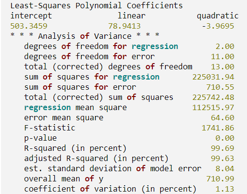
PM, Coefs, Title = 'Least-Squares Polynomial Coefficients'
Least-Squares Polynomial Coefficients
503.346
78.9413
-3.96949
x2 = 9 * FINDGEN(100)/99 - 1
PLOT, x2, coefs(0) + coefs(1) * x2 + coefs(2) * x2^2
OPLOT, x, y, Psym = 1
Example 2
This example is a continuation of the initial example. Here, a procedure is called and defined to output the coefficients and analysis of variance table.
PRO print_results, coefs, anova_table
coef_labels = ['intercept', 'linear', 'quadratic']
PM, coef_labels, coefs, Title = $
'Least-Squares Polynomial Coefficients',$
FORMAT = '(3a20, /,3f20.4, //)'
anova_labels = ['degrees of freedom for regression', $
'degrees of freedom for error', $
'total (corrected) degrees of freedom', $
'sum of squares for regression', $
'sum of squares for error', $
'total (corrected) sum of squares', $
'regression mean square', $
'error mean square', 'F-statistic', $
'p-value', 'R-squared (in percent)', $
'adjusted R-squared (in percent)', $
'est. standard deviation of model error', $
'overall mean of y', 'coefficient of variation (in percent)']
FOR i = 0, 14 DO PM, anova_labels(i), $
anova_table(i), FORMAT = '(a40, f20.2)'
END
x = [0, 0, 1, 1, 2, 2, 4, 4, 5, 5, 6, 6, 7, 7]
y = [508.1, 498.4, 568.2, 577.3, 651.7, $
657.0, 755.3, 758.9, 787.6, 792.1, 841.4, 831.8, 854.7, 871.4]
Coefs = IMSL_POLYREGRESS(x, y, 2, Anova_Table = anova_table)
Least-Squares Polynomial Coefficients
intercept linear quadratic
503.3459 78.9413 -3.9695
Errors
Warning Errors
STAT_CONSTANT_YVALUES: The y values are constant. A zero order polynomial is fit. High order coefficients are set to zero.
STAT_FEW_DISTINCT_XVALUES: There are too few distinct x values to fit the desired degree polynomial. High order coefficients are set to zero.
STAT_PERFECT_FIT: A perfect fit was obtained with a polynomial of degree less than degree. High order coefficients are set to zero.
Fatal Errors
STAT_NONNEG_WEIGHT_REQUEST_2: All weights must be nonnegative.
STAT_ALL_OBSERVATIONS_MISSING: Each (x, y) point contains NaN. There are no valid data.
STAT_CONSTANT_XVALUES: The x values are constant.
Syntax
Result = IMSL_POLYREGRESS(X, Y, Degree [, ANOVA_TABLE=variable] [, DF_PURE_ERROR=variable] [, /DOUBLE] [, PREDICT_INFO=variable] [, RESIDUAL=variable] [, SSQ_LOF=variable] [, SSQ_POLY=variable] [, SSQ_PURE_ERROR=variable] [, WEIGHTS=array] [, XMEAN=variable] [, XVARIANCE=variable])
Return Value
An array of size degree + 1 containing the coefficients of the fitted polynomial.
Arguments
Degree
Degree of the polynomial.
X
One-dimensional array containing the independent variable.
Y
One-dimensional array containing the dependent variable.
Keywords
ANOVA_TABLE (optional)
Named variable into which the analysis of variance table is stored. The analysis of variance statistics are as follows:
- 0: Degrees of freedom for the model
- 1: Degrees of freedom for error
- 2: Total (corrected) degrees of freedom
- 3: Sum of squares for the model
- 4: Sum of squares for error
- 5: Total (corrected) sum of squares
- 6: Model mean square
- 7: Error mean square
- 8: Overall F-statistic
- 9: p-value
- 10: R2 (in percent)
- 11: Adjusted R2 (in percent)
- 12: Estimate of the standard deviation
- 13: Overall mean of y
- 14: Coefficient of variation (in percent)
DF_PURE_ERROR (optional)
Named variable into which the degrees of freedom for pure error is stored.
DOUBLE (optional)
If present and nonzero, double precision is used.
PREDICT_INFO (optional)
Named variable into which the one-dimensional byte array containing information needed by IMSL_POLYPREDICT is stored. The data contained in this array is in an encrypted format and should not be altered before it is used in subsequent calls to IMSL_POLYPREDICT.
RESIDUAL (optional)
Named variable into which the array containing the residuals is stored.
SSQ_LOF (optional)
Named variable into which the array containing the lack-of-fit statistics is stored.
Elements (i, *) correspond to x i+1, i = 0, ..., (degree – 1), and the contents of the array are described in the table that follows.
|
Element |
Description |
|
(i, 0) |
degrees of freedom
|
|
(i, 1) |
lack-of-fit sum of squares
|
|
(i, 2) |
F-statistic for testing lack-of-fit for a polynomial model of degree i
|
|
(i, 3) |
p-value for the test
|
SSQ_POLY (optional)
Named variable into which the array containing the sequential sum of squares and other statistics are stored.
Elements (i, *) correspond to xi+1, i = 0, ..., (degree – 1), and the contents of the array are described in the table that follows:
| Element |
Description |
|
(i, 0) |
degrees of freedom
|
|
(i, 1) |
sum of squares |
|
(i, 2) |
F-statistic
|
|
(i, 3) |
p-value
|
SSQ_PURE_ERROR (optional)
Named variable into which the sum of squares for pure error is stored.
WEIGHTS (optional)
Array containing the vector of weights for the observation. If this option is not specified, all observations have equal weights of 1.
XMEAN (optional)
Named variable into which the mean of x is stored.
XVARIANCE (optional)
Named variable into which the variance of x is stored.
Version History
See Also
IMSL_POLYPREDICT