The IMSL_MULTIPREDICT function computes predicted values, confidence intervals, and diagnostics after fitting a regression model.
This routine requires an IDL Advanced Math and Stats license. For more information, contact your sales or technical support representative.
The general linear model used by IMSL_MULTIPREDICT is:
y = Xβ + ε
where y is the n x 1 vector of responses, X is the n x p matrix of regressors, β is the p x 1 vector of regression coefficients, and ε is the n x 1 vector of errors whose elements are independently normally distributed with mean zero and the following variance:
σ2/wi
From a general linear model fit using the wi’s as the weights, IMSL_MULTIPREDICT computes confidence intervals and statistics for the individual cases that constitute the data set. Let xi be a column vector containing elements of the i-th row of X. Let W = diag(w1, w2, ..., wn). The leverage is defined as hi = (xT (XTWX)–) xi wi. Put D = diag(d1, d2 , ..., dp ) with dj= 1 if the j-th diagonal element of R is positive and zero otherwise.
The leverage is computed as hi = (aTDa)wi, where a is a solution to RTa = xi. The estimated variance of:

is given by the following:
his2/wi, where s2 = SSE/DFE
The computation of the remainder of the case statistics follow easily from their definitions.
Informational errors can occur if the input matrix X is not consistent with the information from the fit (contained in the Predict_info argument), or if excess rounding has occurred. The warning error STAT_NONESTIMABLE arises when X contains a row not in the space spanned by the rows of R. An examination of the model that was fitted and the X for which diagnostics are to be computed is required in order to ensure that only linear combinations of the regression coefficients that can be estimated from the fitted model are specified in X. For further details, see the discussion of estimable functions given in Maindonald (1984, pp. 166–168) and Searle (1971, pp. 180–188).
Often predicted values and confidence intervals are desired for combinations of settings of the independent variables not used in computing the regression fit. This can be accomplished by defining a new data matrix. Since the information about the model fit is input in Predict_info, it is not necessary to send in the data set used for the original calculation of the fit, i.e., only variable combinations for which predictions are desired need be entered in X.
Examples
Example 1
This example calls IMSL_MULTIPREDICT to compute predicted values after calling IMSL_MULTIREGRESS.
x = MAKE_ARRAY(13, 4)
x(0, *) = [7, 26, 6, 60]
x(1, *) = [1, 29, 15, 52]
x(2, *) = [11, 56, 8, 20]
x(3, *) = [11, 31, 8, 47]
x(4, *) = [7, 52, 6, 33]
x(5, *) = [11, 55, 9, 22]
x(6, *) = [3, 71, 17, 6]
x(7, *) = [1, 31, 22, 44]
x(8, *) = [2, 54, 18, 22]
x(9, *) = [21, 47, 4, 26]
x(10, *) = [1, 40, 23, 34]
x(11, *) = [11, 66, 9, 12]
x(12, *) = [10, 68, 8, 12]
y = [78.5, 74.3, 104.3, 87.6, 95.9, 109.2, $
102.7, 72.5, 93.1, 115.9, 83.8, 113.3, 109.4]
coefs = IMSL_MULTIREGRESS(x, y, Predict_Info = predict_info)
predicted = IMSL_MULTIPREDICT(predict_info, x)
PM, predicted, Title = 'Predicted values'
IDL prints:
78.4952
72.7888
105.971
89.3271
95.6492
105.275
104.149
75.6750
91.7216
115.618
81.8090
112.327
111.694
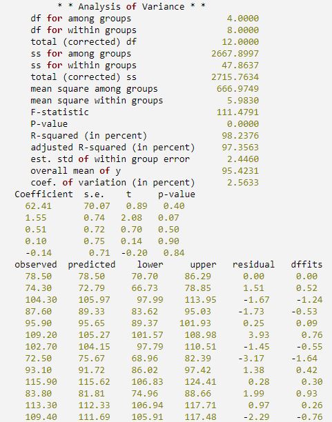
Example 2
This example uses the same data set as the first example and also uses a number of keywords to retrieve additional information from IMSL_MULTIPREDICT. First, a procedure is defined to print the results.
PRO print_results, anova_table, t_tests, y, $
predicted, ci_scheffe, residual, dffits
labels = ['df for among groups ', $
'df for within groups ', $
'total (corrected) df ', $
'ss for among groups ', $
'ss for within groups ', $
'total (corrected) ss ', $
'mean square among groups ', $
'mean square within groups ', $
'F-statistic ', $
'P-value ', $
'R-squared (in percent) ', $
'adjusted R-squared (in percent)', $
'est. std of within group error ', $
'overall mean of y ', $
'coef. of variation (in percent) '] PRINT, ' * * Analysis of Variance * *'
PM, [[labels], [STRING(anova_table, FORMAT = '(f11.4)')]]
PRINT
PRINT, 'Coefficient s.e. t p-value'
PM, t_tests, FORMAT = '(f7.2, 4x, 3f7.2)'
PRINT
PRINT, ' observed predicted lower upper residual dffits'
PM, [[y], [predicted], [transpose(ci_scheffe)], $
[residual], [dffits]], FORMAT = '(6f10.2)'
END
x = MAKE_ARRAY(13, 4)
x(0, *) = [7, 26, 6, 60]
x(1, *) = [1, 29, 15, 52]
x(2, *) = [11, 56, 8, 20]
x(3, *) = [11, 31, 8, 47]
x(4, *) = [7, 52, 6, 33]
x(5, *) = [11, 55, 9, 22]
x(6, *) = [3, 71, 17, 6]
x(7, *) = [1, 31, 22, 44]
x(8, *) = [2, 54, 18, 22]
x(9, *) = [21, 47, 4, 26]
x(10, *) = [1, 40, 23, 34]
x(11, *) = [11, 66, 9, 12]
x(12, *) = [10, 68, 8, 12]
y = [78.5, 74.3, 104.3, 87.6, 95.9, 109.2, $
102.7, 72.5, 93.1, 115.9, 83.8,113.3, 109.4]
coefs = IMSL_MULTIREGRESS(x, y, $
Anova_Table = anova_table, $
T_Tests = t_tests, $
Predict_Info = predict_info, $
Residual = residual)
predicted = IMSL_MULTIPREDICT(predict_info, x, $
Ci_scheffe = ci_scheffe, $
Y = y, $ Dffits = dffits)
print_results, anova_table, t_tests, y, $
predicted, ci_scheffe, residual, dffits
IDL prints:
Errors
Warning Errors
STAT_NONESTIMABLE: Within the preset tolerance, the linear combination of regression coefficients is nonestimable.
STAT_LEVERAGE_GT_1: Leverage (= #) much greater than 1.0 is computed. It is set to 1.0.
STAT_DEL_MSE_LT_0: Deleted residual mean square (= #) much less than zero is computed. It is set to zero.
Fatal Errors
STAT_NONNEG_WEIGHT_REQUEST_2: Weight for row # was #. Weights must be nonnegative.
Syntax
Result = IMSL_MULTIPREDICT(Predict_info, X [, CI_SCHEFFE=variable] [, CI_PTW_POP_MEAN=variable] [, CI_PTW_NEW_SAMP=variable] [, CONFIDENCE=value] [, COOKS_D=variable] [, DEL_RESIDUAL=variable] [, DFFITS=variable] [, /DOUBLE] [, LEVERAGE=variable] [, RESIDUAL=variable] [, STD_RESIDUAL=variable] [, WEIGHTS=array] [, Y=array])
Return Value
One-dimensional array of length N_ELEMENTS (X(*, 0)) containing the predicted values.
Arguments
Predict_info
One-dimensional byte array containing information computed by IMSL_MULTIREGRESS and returned through keyword predict_info. The data contained in this array is in an encrypted format and should not be altered after it is returned by IMSL_MULTIREGRESS.
X
Two-dimensional array containing the combinations of independent variables in each row for which calculations are to be performed.
Keywords
CI_SCHEFFE (optional)
Named variable into which the two-dimensional array of size 2 by N_ELEMENTS (X(*, 0)) containing the Scheffé confidence intervals corresponding to the rows of X is stored. Element Ci_Scheffe (0, i) contains the i-th lower confidence limit; Ci_Scheffe (1, i) contains the i-th upper confidence limit.
CI_PTW_POP_MEAN (optional)
Named variable in the form of a two-dimensional array of size 2 by N_ELEMENTS (X(*, 0)) containing the confidence intervals for two-sided interval estimates of the means, corresponding to the rows of X. Element (0,i) contains the i-th lower confidence limit; Element (1,i) contains the i-th upper confidence limit.
CI_PTW_NEW_SAMP (optional)
Named variable in the form of a two-dimensional array of size 2 by N_ELEMENTS (X(*, 0)) containing the confidence intervals for two-sided prediction intervals, corresponding to the rows of X. Element (0,i) contains the i-th lower confidence limit; Element (1,i) contains the i-th upper confidence limit.
CONFIDENCE
Confidence level for both two-sided interval estimates on the mean and for two-sided prediction intervals, in percent. The value must be in the range [0.0, 100.0). For one-sided intervals with confidence level, where 50.0 ≤ c < 100.0, set CONFIDENCE to 100.0 – 2.0 * (100.0 – c). The default value is 95.0.
COOKS_D (optional)
Named variable in the form of a one-dimensional array of length N_ELEMENTS (X(*, 0)) containing the Cook’s D statistics. You must specify the Y keyword when using this keyword.
DEL_RESIDUAL (optional)
Named variable in the form of a one-dimensional array of length N_ELEMENTS (X(*, 0)) containing the deleted residuals. You must specify the Y keyword when using this keyword.
DFFITS (optional)
Named variable in the form of a one-dimensional array of length N_ELEMENTS (X(*, 0)) containing the DFFITS statistics. You must specify the Y keyword when using this keyword.
DOUBLE (optional)
If present and nonzero, then double precision is used.
LEVERAGE (optional)
Named variable in the form of a one-dimensional array of length N_ELEMENTS (X(*, 0)) containing the leverages.
RESIDUAL (optional)
Named variable in the form of a one-dimensional array of length N_ELEMENTS (X(*, 0)) containing the residuals. You must specify the Y keyword when using this keyword.
STD_RESIDUAL (optional)
Named variable in the form of a one-dimensional array of length N_ELEMENTS (X(*, 0)) containing the standardized residuals. You must specify the Y keyword when using this keyword.
WEIGHTS (optional)
One-dimensional array containing the weight for each row of X. The computed prediction interval uses SSE/(DFE * WEIGHTS(1)) for the estimated variance of a future response. Default: WEIGHTS(*) = 1.
Y (optional)
Array of length N_ELEMENTS (X(*, 0)) containing observed responses.
Version History