The IMSL_MULTIREGRESS function fits a multiple linear regression model, with or without an intercept, using least squares. optionally computes summary statistics for the regression model.
This routine requires an IDL Advanced Math and Stats license. For more information, contact your sales or technical support representative.
By default, the multiple linear regression model is:
yi = β0 + β1xi1 + β2xi2 + ... + βkxik + εi i = 0, 2, ..., n
where the observed values of the yi’s (input in y) are the responses or values of the dependent variable; the xi1’s, xi2’s, ..., xik’s (input in x) are the settings of the k independent variables; β0, β1, ..., βk are the regression coefficients whose estimated values are to be output by IMSL_MULTIREGRESS; and the εi’s are independently distributed normal errors, each with mean zero and variance σ2. Here, n = (N_ELEMENTS(X(*, 0))). Note that by default, β0 is included in the model.
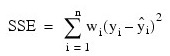
The IMSL_MULTIREGRESS function computes estimates of the regression coefficients by minimizing the weighted sum of squares of the deviations of the observed response yi from the fitted response:

for the n observations. This weighted minimum sum of squares (the error sum of squares) is output as one of the analysis of variance statistics if the ANOVA_TABLE keyword is specified and is computed as shown below:
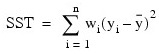
Another analysis of variance statistics is the total sum of squares. By default, the weighted total sum of squares is the weighted sum of squares of the deviations of yi from its mean , the so-called corrected total sum of squares. This statistic is computed as follows:
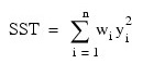
When the NO_INTERCEPT keyword is specified, the total weighted sum of squares is the sum of squares of yi, the so called uncorrected total weighted sum of squares. This is computed as follows:
See Draper and Smith (1981) for a good general treatment of the multiple linear regression model, its analysis, and many examples.
In order to compute a least-squares solution, IMSL_MULTIREGRESS performs an orthogonal reduction of the matrix of regressors to upper-triangular form. The reduction is based on one pass through the rows of the augmented matrix (x,y) using fast Givens transformations (Golub and Van Loan 1983, pp. 156–162; Gentleman 1974). This method has the advantage that it avoids the loss of accuracy that results from forming the crossproduct matrix used in the normal equations.
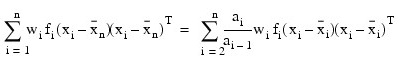
By default, the current means of the dependent and independent variables are used to internally center the data for improved accuracy. Let xj be a column vector containing the j-th row of data for the independent variables. Let represent the mean vector for the independent variables given the data for rows 0, 1,..., i. The current mean vector is defined to be:
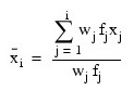
where the wj’s and the fj’s are the weights and frequencies. The i-th row of data hassubtracted from it and is multiplied by:

Although a crossproduct matrix is not computed, the validity of this centering operation can be seen from the formula below for the sum-of-squares and crossproducts matrix:
An orthogonal reduction on the centered matrix is computed. When the final computations are performed, the intercept estimate and the first row and column of the estimated covariance matrix of the estimated coefficients are updated (if COEF_COVARIANCES is specified) to reflect the statistics for the original (uncentered) data. This means that the estimate of the intercept is for the uncentered data.
As part of the final computations, IMSL_MULTIGRESS checks for linearly dependent regressors. In particular, linear dependence of the regressors is declared if any of the following three conditions is satisfied:
- A regressor equals zero.
- Two or more regressors are constant.
- The expression:
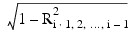
is less than or equal to Tolerance. Here, Ri¥1, 2, ..., i – 1 is the multiple correlation coefficient of the i-th independent variable with the first i – 1 independent variables. If no intercept is in the model, the "multiple correlation" coefficient is computed without adjusting for the mean.
On completion of the final computations, if the i-th regressor is declared to be linearly dependent upon the previous i – 1 regressors, then the i-th coefficient estimate and all elements in the i-th row and i-th column of the estimated variance- covariance matrix of the estimated coefficients (if COEF_COVARIANCES is specified) are set to zero. Finally, if a linear dependence is declared, an error message (code STAT_RANK_DEFICIENT) is issued indicating the model is not full rank.
The IMSL_MULTIREGRESS function also can be used to compute summary statistics from a fitted general linear model. The model is Y = Xβ + ε, where Y is the n x 1 vector of responses, X is the n x p matrix of regressors, β is the p x 1 vector of regression coefficients, and ε is the n x 1 vector of errors whose elements are each independently distributed with mean zero and variance σ2. The IMSL_MULTIREGRESS function uses the results of this fit to compute summary statistics, including analysis of variance, sequential sum of squares, t tests, and an estimated variance-covariance matrix of the estimated regression coefficients.
Some generalizations of the general linear model are allowed. If the i-th element of ε has a variance of:\

and the weights wi are used in the fit of the model, IMSL_MULTIREGRESS produces summary statistics from the weighted least-squares fit. More generally, if the variance-covariance matrix of ε is σ2V, IMSL_MULTIREGRESS can be used to produce summary statistics from the generalized least-squares fit. The
IMSL_MULTIREGRESS function can be used to perform a generalized least-squares fit by regressing Y* on X* where Y* = (T –1)TY, X* = (T –1)TX, and T satisfies TTT = V.
The sequential sum of squares for the i-th regression parameter is given by:

The regression sum of squares is given by the sum of the sequential sum of squares. If an intercept is in the model, the regression sum of squares is adjusted for the mean, i.e.:
is not included in the sum.
The estimate of σ2 is s2 (stored in ANOVA_TABLE(7)) that is computed as SSE/DFE.
If R is nonsingular, the estimated variance-covariance matrix of  (stored in Coef_Covariances) is computed by s2R –1(R –1)T.
If R is singular, corresponding to rank(X) < p, a generalized inverse is used. For a matrix G to be a gi (i = 1, 2, 3, or 4) inverse of a matrix A, G must satisfy conditions j (for j ≤ i) for the Moore-Penrose inverse but generally must fail conditions k (for k > i).
The four conditions for G to be a Moore-Penrose inverse of A are as follows:
- AGA = A
- GAG = G
- AG is symmetric
-
GA is symmetric
In the case where R is singular, the method for obtaining COEF_COVARIANCES follows the discussion of Maindonald (1984, pp. 101–103). Let Z be the diagonal matrix with diagonal elements defined by the following:
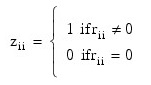
Let G be the solution to RG = Z obtained by setting the i-th ({i:rii = 0}) row of G to zero. The keyword COEF_COVARIANCES is set to s2GGT. (G is a g3 inverse of R, represented by Rg3. The result Rg3Rg3T is a symmetric g2 inverse of RTR = XTX. See Sallas and Lionti 1988.)
The keyword COEF_COVARIANCES can only be used to get variances and covariances of estimable functions of the regression coefficients. In other words, nonestimable functions (linear combinations of the regression coefficients not in the space spanned by the nonzero rows of R) must not be used. See, for example, Maindonald (1984, pp. 166–168) for a discussion of estimable functions.
The estimated standard errors of the estimated regression coefficients (stored in Column 1 of T_TESTS) are computed as square roots of the corresponding diagonal entries in COEF_COVARIANCES.
For the case where an intercept is in the model, set  equal to the matrix R with the first row and column deleted. Generally, the variance inflation factor (VIF) for the i-th regression coefficient is computed as the product of the i-th diagonal element of RTR and the i-th diagonal element of its computed inverse. If an intercept is in the model, the VIF for those coefficients not corresponding to the intercept uses the diagonal elements of:

See Maindonald (1984), p. 40.
Remarks
When R is nonsingular and comes from an unrestricted regression fit, COEF_COVARIANCES is the estimated variance-covariance matrix of the estimated regression coefficients and COEF_COVARIANCES = (SSE/DFE) (RTR) – 1.
Otherwise, variances and covariances of estimable functions of the regression coefficients can be obtained using COEF_COVARIANCES and COEF_COVARIANCES = (SSE/DFE) (GDGT). Here, D is the diagonal matrix with diagonal elements equal to zero if the corresponding rows of R are restrictions and with diagonal elements equal to 1 otherwise. Also, G is a particular generalized inverse of R.
Examples
Example 1
A regression model:
yi = β0 + β1xi1 + β2xi2 + ... + β3xi3 + εi i = 1, 2, ..., 9
is fitted to data taken from Maindonald (1984, pp. 203–204).
RM, x, 9, 3
row 0: 7 5 6
row 1: 2 -1 6
row 2: 7 3 5
row 3: -3 1 4
row 4: 2 -1 0
row 5: 2 1 7
row 6: -3 -1 3
row 7: 2 1 1
row 8: 2 1 4
y = [7, -5, 6, 5, 5, -2, 0, 8, 3]
coefs = IMSL_MULTIREGRESS(x, y)
PM, coefs, TITLE = 'Least-Squares Coefficients', $
FORMAT = '(f10.5)'
IDL prints:
Least-Squares Coefficients
7.73333
-0.20000
2.33333
-1.66667
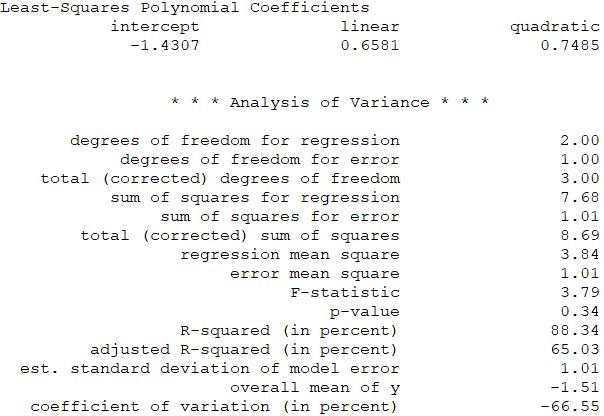
Example 2: Weighted Least-squares Fit
A weighted least-squares fit is computed using the model:
yi = β0 + β1xi1 + β2xi2 + εi i = 1, 2, ..., 4
and weights 1/i2 discussed by Maindonald (1984, pp. 67–68).
In the example, the WEIGHTS keyword is specified. The minimum sum of squares for error in terms of the original untransformed regressors and responses for this weighted regression is:
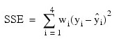
where wi = 1/i2, represented in the C code as array w.
A procedure is defined to output the results, including the analysis of variance statistics:
PRO print_results, Coefs, Anova_Table
coef_labels = ['intercept', 'linear', 'quadratic']
PM, coef_labels, coefs, TITLE = $
'Least-Squares Polynomial Coefficients', $
FORMAT = '(3a20, /,3f20.4, // )'
anova_labels = ['degrees of freedom for regression', $
'degrees of freedom for error', $
'total (corrected) degrees of freedom', $
'sum of squares for regression', $
'sum of squares for error', $
'total (corrected) sum of squares', $
'regression mean square', $
'error mean square', 'F-statistic', $
'p-value', 'R-squared (in percent)', $
'adjusted R-squared (in percent)', $
'est. standard deviation of model error', $
'overall mean of y', $
'coefficient of variation (in percent)']
PM, '* * * Analysis of Variance * * * ', FORMAT = '(a50, /)'
FOR i = 0, 14 DO PM, anova_labels(i), $
anova_table(i), FORMAT = '(a40, f20.2)'
END
RM, x, 4, 2
row 0: -2 0
row 1: -1 2
row 2: 2 5
row 3: 7 3
y = [-3.0, 1.0, 2.0, 6.0]
weights = FLTARR(4)
FOR i = 0, 3 DO weights(i) = 1/((i + 1.0)^2)
PM, weights
IDL prints:
1.00000
0.250000
0.111111
0.0625000
coefs = IMSL_MULTIREGRESS(x, y, WEIGHTS = weights, $
ANOVA_TABLE = anova_table)
print_results, coefs, anova_table
IDL prints:
Example 3: Plotting Results
This example uses IMSL_MULTIREGRESS to fit data with both simple linear regression and second order regression. The results are plotted along with confidence bands and residual plots.
PRO IMSL_MULTIREGRESS_ex
!P.MULTI = [0, 2, 2]
x = [1.0, 1.0, 2.0, 2.0, 3.0, 3.0, 4.0, 4.0, 5.0, 5.0]
y = [1.1, 0.1, -1.2, 0.3, 1.4, 2.6, 3.1, 4.2, 9.3, 9.6]
z = FINDGEN(120)/20
line = MAKE_ARRAY(120, VALUE = 0.0)
Coefs = IMSL_MULTIREGRESS(x, y, PREDICT_INFO = predict_info)
y_hat = IMSL_MULTIPREDICT(predict_info, x, $
RESIDUAL = residual, Y = y)
y_hat = IMSL_MULTIPREDICT(predict_info, z, $
CI_PTW_NEW_SAMP = ci)
PLOT, x, y, Title = 'Simple linear regression', $
PSYM = 4, XRANGE = [0.0, 6.0]
y2 = coefs(0) + coefs(1) * z
OPLOT, z, y2
OPLOT, z, ci(0, *), LINESTYLE = 1
OPLOT, z, ci(1, *), LINESTYLE = 1
PLOT, x, residual, PSYM = 4, TITLE = $
'Residual plot for simple linear regression', $
XRANGE = [0.0, 6.0], YRANGE = [-6, 6]
x2 = [[x], [x * x]]
coefs = IMSL_MULTIREGRESS(x2, y, PREDICT_INFO = predict_info)
y_hat = IMSL_MULTIPREDICT(predict_info, x2, $ RESIDUAL = residual, Y = y)
y_hat = IMSL_MULTIPREDICT(predict_info, $
[[z], [z * z]], CI_PTW_NEW_SAMP = ci)
PLOT, x, y, Title = '2nd order regression', $
PSYM = 4, XRANGE = [0.0, 6.0]
y2 = coefs(0) + coefs(1) * z + coefs(2) * z * z OPLOT, z, y2
OPLOT, z, ci(0, *), LINESTYLE = 1
OPLOT, z, ci(1, *), LINESTYLE = 1
PLOT, x2, residual, PSYM = 4, TITLE = $
'Residual plot for 2nd order regression', $
XRANGE = [0.0, 6.0], YRANGE = [-6, 6]
OPLOT, z, line
END
Result:
Example 4: Two-variable, Second-degree Fit
In this example, IMSL_MULTIREGRESS is used to compute a two variable second- degree fit to data.
PRO IMSL_MULTIREGRESS_ex
x1(*, 0) = [8.5, 8.9, 10.6, 10.2, 9.8, $
10.8, 11.6, 12.0, 12.5, 10.9]
x1(*, 1) = [2, 3, 3, 20, 22, 20, 31, 32, 31, 28]
x1(*, 2) = x1(*, 0) * x1(*, 1)
x1(*, 3) = x1(*, 0) * x1(*, 0)
x1(*, 4) = x1(*, 1) * x1(*, 1)
y = [30.9, 32.7, 36.7, 41.9, 40.9, 42.9, 46.3, 47.6, 47.2, 44.0]
nxgrid = 30
nygrid = 30
ax1 = min(x1(*, 0)) + (max(x1(*, 0)) - $
min(x1(*, 0))) * FINDGEN(nxgrid)/(nxgrid - 1)
ax2 = MIN(x1(*, 1)) + (MAX(x1(*, 1)) - $
MIN(x1(*, 1))) * FINDGEN(nxgrid)/(nxgrid - 1)
coefs = IMSL_MULTIREGRESS(x1, y, RESIDUAL = resid)
z = FLTARR(nxgrid, nygrid)
FOR i = 0, nxgrid - 1 DO BEGIN
FOR j = 0, nygrid-1 DO BEGIN
z(i,j) = Coefs(0) $
+ Coefs(1) * ax1(i) + Coefs(2) * ax2(j) $
+ Coefs(3) * ax1(i) * ax2(j) $
+ Coefs(4) * ax1(i)^2 $
+ Coefs(5) * ax2(j)^2
ENDFOR
ENDFOR
!P.CHARSIZE = 2
SURFACE, z, ax1, ax2, /SAVE, XTITLE = 'X1', YTITLE = 'X2'
PLOTS, x1(*, 0), x1(*, 1), y, /T3D, PSYM = 4, SYMSIZE = 3
XYOUTS, .3, .9, /NORMAL, 'Two-Variable Second-Degree Fit'
END
Result:
Errors
Warning Errors
STAT_RANK_DEFICIENT: Model is not full rank. There is not a unique least- squares solution.
Syntax
Result = IMSL_MULTIREGRESS(X, Y [, ANOVA_TABLE=variable] [, COEF_COVARIANCES=variable] [, COEF_VIF=variable] [, /DOUBLE] [, FREQUENCIES=array] [, /NO_INTERCEPT] [, PREDICT_INFO=variable] [, RANK=variable] [, RESIDUAL=variable] [, T_TESTS=variable] [, TOLERANCE=value] [, WEIGHTS=array] [, XMEAN=variable])
Return Value
If the keyword NO_INTERCEPT is not used, the result is an array of length N_ELEMENTS (X(*, 0)) containing a least-squares solution for the regression coefficients. The estimated intercept is the initial component of the array.
Arguments
X
Two-dimensional matrix containing the independent (explanatory) variables. The data value for the i-th observation of the j-th independent (explanatory) variable should be in element X(i, j).
Y
Two-dimensional matrix containing of size N_ELEMENTS(X(*,0)) by the number of dependent variables, containing the dependent (response) variable(s). The i-th column of y contains the i-th dependent variable.
Keywords
ANOVA_TABLE (optional)
Named variable into which the analysis of variance table is stored. The analysis of variance statistics are as follows:
- 0: Degrees of freedom for the model
- 1: Degrees of freedom for error
- 2: Total (corrected) degrees of freedom
- 3: Sum of squares for the model
- 4: Sum of squares for error
- 5: Total (corrected) sum of squares
- 6: Model mean square
- 7: Error mean square
- 8: Overall F-statistic
- 9: p-value
- 10: R2 (in percent)
- 11: Adjusted R2 (in percent)
- 12: Estimate of the standard deviation
- 13: Overall mean of y
- 14: Coefficient of variation (in percent)
COEF_COVARIANCES (optional)
Named variable with an m x m x n_dependent array containing estimated variances and covariances of the estimated regression coefficients. Here, m is number of regression coefficients in the model. If NO_INTERCEPT is specified, m = N_ELEMENTS(X(0, *)); otherwise, m = (N_ELEMENTS(X(0, *)) + 1).
COEF_VIF (optional)
Named variable in the form of a one-dimensional array of length NPAR containing the variance inflation factor. NPAR is the number of parameters. The (i + INTCEP)-th element corresponds to the i-th independent variable, where i = 0, 1, 2,..., NPAR – 1. INTCEP is equal to 1 if an intercept is in the model and 0 otherwise. The square of the multiple correlation coefficient for the i-th regressor after all others is obtained from Coef_Vif by the following formula:

If there is no intercept or there is an intercept and i = 0, the multiple correlation coefficient is not adjusted for the mean.
DOUBLE (optional)
If present and nonzero, then double precision is used.
FREQUENCIES (optional)
One-dimensional array containing the frequency for each observation. Default: Frequencies(*) = 1.
NO_INTERCEPT (optional)
If present and nonzero, the intercept term  is omitted from the model. By default, the fitted value for observation i is:
where k is the number of independent variables.
PREDICT_INFO (optional)
Named variable in the form of a one-dimensional byte array containing information needed by IMSL_MULTIPREDICT. The data contained in this array is in an encrypted format and should not be altered before it is used in subsequent calls to IMSL_MULTIPREDICT.
RANK (optional)
Named variable containing the rank of the fitted model.
RESIDUAL (optional)
Variable with an array containing the residuals.
T_TESTS (optional)
Named variable with an NPAR by 4 array containing statistics relating to the regression coefficients. NPAR is equal to the number of parameters in the model. Each row corresponds to a coefficient in the model. Row i + INTCEP corresponds to the i-th independent variable, and i = 0, 1, 2, ..., NPAR – 1. INTCEP is equal to 1 if an intercept is in the model and 0 otherwise. The statistics in the columns are as follows:
- 0: coefficient estimate
- 1: estimated standard error of the coefficient estimate
- 2: t-statistic for the test that the coefficient is 0
- 3: p-value for the two-sided t test
TOLERANCE (optional)
Tolerance used in determining linear dependence. The default value is 100 x ε, where ε is machine precision.
WEIGHTS (optional)
One-dimensional array containing the weight for each observation. Default: Weights(*) = 1.
XMEAN (optional)
Named variable with an array containing the estimated means of the independent variables.
Version History