The IMSL_POISSON2D function solves Poisson’s or Helmholtz’s equation on a two-dimensional rectangle using a fast Poisson solver based on the HODIE finite- difference scheme on a uniform mesh.
This routine requires an IDL Advanced Math and Stats license. For more information, contact your sales or technical support representative.
Let c = Coef_U, ax = ax, bx = bx, ay = ay, by = by, nx = nx and ny = ny.
IMSL_POISSON2D is based on the code HFFT2D by Boisvert (1984). It solves the equation:
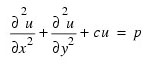
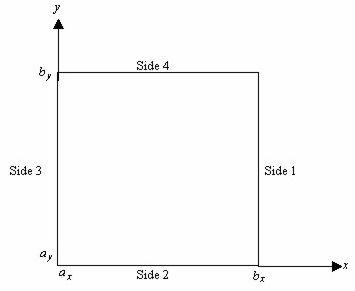
on the rectangular domain (ax, bx) x (ay, by)) with a user-specified combination of Dirichlet (solution prescribed), Neumann (first-derivative prescribed), or periodic boundary conditions. The sides are numbered clockwise, starting with the right side, as shown in the following figure.
When c = 0 and only Neumann or periodic boundary conditions are prescribed, then any constant may be added to the solution to obtain another solution to the problem. In this case, the solution of minimum ∞-norm is returned.
The solution is computed using either a second-or fourth-order accurate finite- difference approximation of the continuous equation. The resulting system of linear algebraic equations is solved using fast Fourier transform techniques. The algorithm relies on the fact that nx – 1 is highly composite (the product of small primes). For details of the algorithm, see Boisvert (1984). If nx – 1 is highly composite then the execution time of IMSL_POISSON2D is proportional to nxny log2 nx. If evaluations of p(x, y) are inexpensive, then the difference in running time between ORDER = 2 and ORDER = 4 is small.
The grid spacing is the distance between the (uniformly spaced) grid lines. It is given by the formulas hx = (bx – ax)/(nx – 1) and hy = (by – ay)/(ny – 1). The grid spacings in the x and y directions must be the same, i.e., nx and ny must be such that hx is equal to hy. Also, as noted above, nx and ny must be at least 4. To increase the speed of the fast Fourier transform, nx – 1 should be the product of small primes. Good choices are 17, 33, and 65.
If –coef_u is nearly equal to an eigenvalue of the Laplacian with homogeneous boundary conditions, then the computed solution might have large errors.
Example
This example solves the equation:
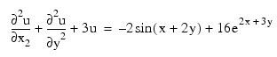
with the boundary conditions:
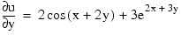
on the bottom side and:
on the other three sides. The domain is the rectangle [0, 1/4] x [0, 1/2]. The output of IMSL_POISSON2D is a 17 x 33 table of values. The functions IMSL_SPVALUE are used to print a different table of values.
FUNCTION rhs_pde, x, y
f = (-2.0*SIN(x + 2.0*y) + 16.0*EXP(2.0*x + 3.0*y))
RETURN, f
END
FUNCTION rhs_bc, side, x, y
IF (side EQ 1) THEN $
f = 2.0*COS(x + 2.0*y) + 3.0*EXP(2.0*x + 3.0*y) $
ELSE $
f = SIN(x + 2.0*y) + EXP(2.0*x + 3.0*y)
RETURN, f
END
PRO print_results, x, y, utable
FOR j = 0, 4 DO FOR i = 0, 4 DO $
PRINT, x(i), y(j), utable(i, j), $
ABS(utable(i, j) - SIN(x(i) + 2.0*y(j)) - $
EXP(2.0*x(i) + 3.0*y(j)))
END
nx = 17
nxtable = 5
ny = 33
nytable = 5
ax = 0.0
bx = 0.25
ay = 0.0
by = 0.5
bc_type = [1, 2, 1, 1]
coef_u = 3.0
u = IMSL_POISSON2D('rhs_pde', 'rhs_bc', coef_u, nx, ny, ax, $
bx, ay, by, bc_type)
xdata = ax + (bx - ax)*FINDGEN(nx)/(nx - 1)
ydata = ay + (by - ay)*FINDGEN(ny)/(ny - 1)
sp = IMSL_BSINTERP(xdata, ydata, u)
x = ax + (bx - ax)*FINDGEN(nxtable)/(nxtable - 1)
y = ay + (by - ay)*FINDGEN(nytable)/(nytable - 1)
utable = IMSL_SPVALUE(x, y, sp)
PRINT,' X Y U Error'
print_results, x, y, utable
END
IDL prints:
X Y U Error
0.00000 0.00000 1.00000 0.00000
0.0625000 0.00000 1.19560 4.88758e-06
0.125000 0.00000 1.40869 7.39098e-06
0.187500 0.00000 1.64139 4.88758e-06
0.250000 0.00000 1.89613 1.19209e-07
0.00000 0.125000 1.70240 1.19209e-07
0.0625000 0.125000 1.95615 6.55651e-06
0.125000 0.125000 2.23451 9.53674e-06
0.187500 0.125000 2.54067 6.67572e-06
0.250000 0.125000 2.87830 0.00000
0.00000 0.250000 2.59643 4.76837e-07
0.0625000 0.250000 2.93217 9.05991e-06
0.125000 0.250000 3.30337 1.31130e-05
0.187500 0.250000 3.71482 8.82149e-06
0.250000 0.250000 4.17198 2.38419e-07
0.00000 0.375000 3.76186 2.38419e-07
0.0625000 0.375000 4.21634 9.05991e-06
0.125000 0.375000 4.72261 1.31130e-05
0.187500 0.375000 5.28776 8.58307e-06
0.250000 0.375000 5.91989 4.76837e-07
0.00000 0.500000 5.32316 4.76837e-07
0.0625000 0.500000 5.95199 0.00000
0.125000 0.500000 6.65687 4.76837e-07
0.187500 0.500000 7.44826 0.00000
0.250000 0.500000 8.33804 1.43051e-06
Syntax
Result = IMSL_POISSON2D(Rhs_Pde, Rhs_Bc, Coef_U, Nx, Ny, Ax, Bx, Ay, By, Bc_Type [, /DOUBLE] [, ORDER=value])
Return Value
Two-dimensional array of size nx by ny containing solution at the grid points.
Arguments
Rhs_Pde
Scalar string specifying the name of the user-supplied function to evaluate the right-hand side of the partial differential equation at a scalar value x and scalar value y.
Rhs_Bc
Scalar string specifying the name of the user-supplied function to evaluate the right-hand side of the boundary conditions, on side side, at scalar value x and scalar value y. The value of side will be one of the integer values shown below.
|
Integer |
Side |
|
0 |
right side |
|
1 |
bottom side |
|
2 |
left side |
|
3 |
top side |
Coef_U
Value of the coefficient of u in the differential equation.
Nx
Number of grid lines in the x-direction. nx must be at least 4. See the description at the beginning of this topic for further restrictions on nx.
Ny
Number of grid lines in the y-direction. nx must be at least 4. See the description at the beginning of this topic for further restrictions on ny.
Ax
The value of x along the left side of the domain.
Bx
The value of x along the right side of the domain.
Ay
The value of y along the bottom of the domain.
By
The value of y along the top of the domain.
Bc_Type
One-dimensional array of size 4 indicating the type of boundary condition on each side of the domain or that the solution is periodic. The sides are numbered as shown below.
|
Array |
Side |
Location |
|
Bc_Type(0)
|
right |
x = bx |
|
Bc_Type(1)
|
bottom |
y = ay |
|
Bc_Type(2)
|
left |
x = ax |
|
Bc_Type(3)
|
top |
y = by |
The three possible boundary condition types are shown below.
|
Type |
Condition |
|
Bc_Type(i) = 1
|
Dirichlet condition. Value of u is given.
|
|
Bc_Type(i) = 2
|
Neuman condition. Value of du/dx is given (on the right or left sides) or du/dy (on the bottom or top of the domain).
|
|
Bc_Type(i) = 3
|
Periodic condition.
|
Keywords
DOUBLE (optional)
If present and nonzero, then double precision is used.
ORDER (optional)
Order of accuracy of the finite-difference approximation. It can be either 2 or 4. Default: 4
Version History
See Also
IMSL_POISSONCDF