The IMSL_RADBF function computes an approximation to scattered data in Rn for n ≥ 2 using radial-basis functions.
This routine requires an IDL Advanced Math and Stats license. For more information, contact your sales or technical support representative.
The IMSL_RADBF function computes a least-squares fit to scattered data in Rd. More precisely, let n = N_ELEMENTS (fdata), x = abscissa, f = fdata, and d = N_ELEMENTS (abscissa (0, *)). Then:
This function computes a function F which approximates the above data in the sense that it minimizes the sum-of-squares error:

where w = WEIGHTS.
The functional form of F is restricted as follows:
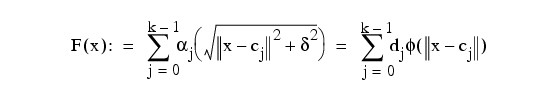
The function φ is called the radial function. It maps R1 into R1. It needs to be defined only for the nonnegative reals. For the purpose of this routine, the user supplied a function:
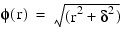
Note that the value of delta is defaulted to 1. It can be set by the user by using keyword Delta.
The default-basis function is called the Hardy multiquadric and is defined as:
A key feature of this routine is the user’s control over the selection of the basis function.
In order to obtain the default selection of centers, first compute the number of centers that will be on a grid and the number that will be on a random subset of the Abscissa. Next, compute those centers on a grid. Finally, a random subset of Abscissa is obtained. This determines where the centers are placed. The selection of centers is discussed in more detail below.
First, the computed grid is restricted to have the same number of grid values in each of the dimension directions. Then, the number of centers placed on a grid, num_gridded, is computed as follows:

Note that there are β grid values in each of the dimension directions. Then:
num_random = (num_centers) – (num_gridded)
How many centers are placed on a grid and how many are placed on a random subset of the abscissa is now known. The gridded centers are computed such that they are equally spaced in each of the dimension directions. The last problem is to compute a random subset, without replacement, of the abscissa. The selection is based on a random seed. The default seed is 234579. The user can change this using optional keyword RANDOM_SEED. Once the subset is computed, the Abscissa as centers is used.
Since the selection of good centers for a specific problem is an unsolved problem at this time, ultimate flexibility is given to the user; that is, the user can select centers using keyword CENTERS. As a rule of thumb, the centers should be interspersed with the Abscissa.
The return value for this function is a pointer to the structure containing all the information necessary to evaluate the fit. This pointer is then passed to the IMSL_RADBE function to produce values of the fitted function.
Examples
Example 1
Fitting Noisy Data with Default Radial Function
In this example, IMSL_RADBF is used to fit noisy data. Four plots are generated using different values for num_centers as shown in the figure that follows. The plots generated by running this example are included after the code. Note that the triangles represent the placement of the centers.
PRO radbf_ex1
!P.Multi = [0, 2, 2]
ndata = 10 noise_size = .05
xydata = DBLARR(1, ndata)
fdata = DBLARR(ndata)
noise = 1 - 2 * IMSL_RANDOM(ndata, /Double)
xydata(0, *) = 15 * IMSL_RANDOM(ndata)
fdata = REFORM(COS(xydata(0, *)) + noise_size * noise, ndata)
FOR i = 0, 3 DO BEGIN
num_centers = ndata/3 + i
radial_struct = IMSL_RADBF(xydata, fdata, num_centers)
a(0, *) = 15 * FINDGEN(100)/99.
fit = IMSL_RADBE(a, radial_struct)
title = 'Fit with NUM_CENTERS = ' + $
STRCOMPRESS(num_centers, /Remove_All)
PLOT, xydata(0, *), fdata, Title = title, $
Psym = 6, Yrange = [-1.25, 1.25]
OPLOT, radial_struct.CENTERS, $
MAKE_ARRAY(num_centers, Value=-1.25), Psym = 5
END
END
Example 2
Fitting Noisy Data with User-supplied Radial Function
This example fits the same data as the first example, but the user supplies the radial function and sets RATIO_CENTERS to zero. The radial function used in this example is φ (r) = ln (1 + r2). Four plots are generated using different values for Num_Centers as shown in the figure that follows. The plots generated by running this example are included after the code. Note that the triangles represent the placement of the centers.
FUNCTION user_fcn, distance
END
PRO radbf_ex2
!P.Multi = [0, 2, 2]
ndata = 10 noise_size = .05
xydata = DBLARR(1, ndata) fdata = DBLARR(ndata)
IMSL_RANDOMOPT, Set = 234579
noise = 1 - 2 * IMSL_RANDOM(ndata, /Double)
xydata(0, *) = 15 * IMSL_RANDOM(ndata)
fdata = REFORM(COS(xydata(0,*)) + noise_size * noise, ndata)
FOR i = 0, 3 DO BEGIN
radial_struct = IMSL_RADBF(xydata, fdata, $
num_centers, Ratio_Centers = 0, Basis = 'user_fcn')
a(0, *) = 15 * FINDGEN(100)/99.
fit = IMSL_RADBE(a, radial_struct)
title = 'Fit with NUM_CENTERS = ' + $
STRCOMPRESS(num_centers, /Remove_All)
PLOT, xydata(0,*), fdata, Title = title, $
Psym = 6, Yrange = [-1.25, 1.25]
OPLOT, a(0, *), fit
OPLOT, radial_struct.CENTERS, $
MAKE_ARRAY(num_centers,Value = -1.25), Psym = 5
END
END
Figure 6-17: Fit using a User-Defined Radial Function
Example 3: Fitting a Surface to Three-dimensional Scattered Data
This example fits a surface to scattered data. The scattered data is generated using the function f (x, y) = exp (ln (y + 1) sin (x)). The plots generated by running this example are included after the code as shown in the figures that follow.
FUNCTION f, x1, x2
RETURN, EXP(ALOG10(x2 + 1)) * SIN(x1)
END
PRO radbf_ex3
IMSL_RANDOMOPT, Set = 123457
ndata = 50 num_centers = ndata
xydata = DBLARR(2, ndata)
fdata = DBLARR(ndata)
xrange = 8 yrange = 5
xydata(0,*) = xrange * IMSL_RANDOM(ndata, /Double)
xydata(1,*) = yrange * IMSL_RANDOM(ndata, /Double)
fdata(*) = f(xydata(0, *), xydata(1, *))
radial_struct = IMSL_RADBF(xydata, fdata, num_centers, Ratio=0)
nx = 25
ny = 25
xyfit = DBLARR(2, nx * ny)
xyfit(0, *) = xrange * (FINDGEN(nx * ny)/ny)/(nx - 1)
xyfit(1, *) = yrange * (FINDGEN(nx * ny) MOD ny)/(ny - 1)
zfit = TRANSPOSE(REFORM(IMSL_RADBE(xyfit, Radial_Struct), $
ny, nx))
xt = xrange * FINDGEN(nx)/(nx-1)
yt = yrange * FINDGEN(ny)/(ny-1)
SURFACE, zfit, xt, yt, /Save, Zrange = [MIN(zfit), MAX(zfit)]
PLOTS, xydata(0, *), xydata(1, *), fdata, $
/T3d, Psym = 4, Symsize = 2
WINDOW, /Free
orig = DBLARR(nx, ny)
FOR i = 0, (nx-1) DO FOR j = 0, (ny-1) DO $
orig(i, j) = f(xt(i), yt(j))
SURFACE, orig, xt, yt, Zrange = [MIN(zfit), MAX(zfit)]
END
Syntax
Result = IMSL_RADBF(Abscissa, Fdata, Num_Centers [, BASIS=string] [, CENTERS=value] [, DELTA=value] [, /DOUBLE] [, RANDOM_SEED=value] [, RATIO_CENTERS=value] [, WEIGHTS=value])
Return Value
A structure that represents the radial-basis fit.
Arguments
Abscissa
Two-dimensional array containing the abscissas of the data points. Parameter abscissa (i, j) is the Abscissa value of the j-th data point in the i-th dimension.
Fdata
One-dimensional array containing the ordinates for the problem.
Num_Centers
Number of centers to be used when computing the radial-basis fit. The Num_Centers argument should be less than or equal to N_ELEMENTS (Fdata).
Keywords
BASIS (optional)
Character string specifying a user-supplied function to compute the values of the radial functions. The form of the input function is ϕ (r). Default: the Hardy multiquadratic.
CENTERS (optional)
User-supplied centers. See the discussion section for details.
DELTA (optional)
Delta used in the default basis function, φ (r) = SQRT(r2 + δ2). Default: 1.
DOUBLE (optional)
If present and nonzero, double precision is used.
RANDOM_SEED (optional)
Value of the random seed used when determining the random subset of abscissa to use as centers. By changing the value of seed on different calls to IMSL_RADBF, with the same data set, a different set of random centers are chosen. Setting RANDOM_SEED to zero forces the random number seed to be based on the system clock, so possibly, a different set of centers is chosen each time the program is executed. Default: 234579.
RATIO_CENTERS (optional)
Desired ratio of centers placed on an evenly spaced grid to the total number of centers. There is a condition: The same number of centers placed on a grid for each dimension must be equal. Thus, the actual number of centers placed on a grid is usually less than RATIO_CENTERS * Num_Centers, but is never more than RATIO_CENTERS * Num_Centers. The remaining centers are randomly chosen from the set of abscissa given in abscissa. Default: 0.5
WEIGHTS (optional)
Requires the user to provide the weights. Default: all weights equal 1.
Version History
See Also
IMSL_RADBE