The IMSL_ANOVAFACT function analyzes a balanced factorial design with fixed effects.
This routine requires an IDL Advanced Math and Stats license. For more information, contact your sales or technical support representative.
The IMSL_ANOVAFACT function performs an analysis for an n-way classification design with balanced data. For balanced data, there must be an equal number of responses in each cell of the n-way layout. The effects are assumed to be fixed effects. The model is an extension of the two-way model to include n factors. The interactions (two-way, three-way, up to n-way) can be included in the model, or some of the higher-way interactions can be pooled into error. The keyword Order specifies the number of factors to be included in the highest-way interaction. For example, if three-way and higher-way interactions are to be pooled into error, set Order = 2.
By default, Order = N_ELEMENTS (n_levels) – 1 with the last subscript being the replicates subscript. Keyword Pure_Error indicates there are repeated responses within the n-way cell; Pool_Inter indicates otherwise.
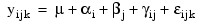
The IMSL_ANOVAFACT function requires the responses as input into a single vector y in lexicographical order, so that the response subscript associated with the first factor varies least rapidly, followed by the subscript associated with the second factor, and so forth. Hemmerle (1967, Chapter 5) discusses the computational method.
Examples
Example 1
A two-way analysis of variance is performed with balanced data discussed by Snedecor and Cochran (1967, Table 12.5.1, p. 347). The responses are the weight gains (in grams) of rats that were fed diets varying in the source (A) and level (B) of protein.
The model is:
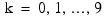
for


where
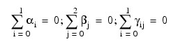
for
and

for i = 0, 1. The first responses in each cell in the two-way layout are given in the table that follows.
|
Protein Level (B)
|
Protein Source (A)
|
|
Beef |
Cereal |
Pork |
|
High |
73, 102, 118, 104, 81, 107, 100, 87, 117, 111
|
98, 74, 56, 111, 95, 88, 82, 77, 86, 92
|
94, 79, 96, 98, 102, 102, 108, 91, 120, 105
|
|
Low |
90, 76, 90, 64, 86, 51, 72, 90, 95, 78
|
107, 95, 97, 80, 98, 74, 74, 67, 89, 58
|
49, 82, 73, 86, 81, 97, 106, 70, 61, 82
|
n = [3, 2, 10]
y = [73.0, 102.0, 118.0, 104.0, 81.0, $
107.0, 100.0, 87.0, 117.0, 111.0, $
90.0, 76.0, 90.0, 64.0, 86.0, $
51.0, 72.0, 90.0, 95.0, 78.0, $
98.0, 74.0, 56.0, 111.0, 95.0, $
88.0, 82.0, 77.0, 86.0, 92.0, $
107.0, 95.0, 97.0, 80.0, 98.0, $
74.0, 74.0, 67.0, 89.0, 58.0, $
94.0, 79.0, 96.0, 98.0, 102.0, $
102.0, 108.0, 91.0, 120.0, 105.0, $
49.0, 82.0, 73.0, 86.0, 81.0, $
97.0, 106.0, 70.0, 61.0, 82.0]
p_value = IMSL_ANOVAFACT(n, y, Anova_Table = anova_table)
PRINT, 'p-value = ', p_value
IDL prints:
p-value = 0.00229943
Example 2: Two-way ANOVA
In this example, the same model and data are fit as in the initial example, but keywords are used for a more complete analysis. First, a procedure to output the results is defined.
.RUN
PRO print_results, anova_table, test_effects, means
anova_labels = ['df for among groups', $
'df for within groups', 'total (corrected) df', $
'ss for among groups', 'ss for within groups', $
'total (corrected) ss', 'mean square among groups', $
'mean square within groups', 'F-statistic', $
'P-value', 'R-squared (in percent)', $
'adjusted R-squared (in percent)', $
'est. std of within group error', 'overall mean of y', $
'coef. of variation (in percent)']
effects_labels = ['A ', 'B ', 'A*B']
means_labels = ['grand', 'A1', 'A2', $
'A3', 'B1', 'B2', 'A1*B1', 'A1*B2', $
'A2*B1', 'A2*B2', 'A3*B1', 'A3*B2']
PRINT, ' * *Analysis of Variance * *'
FOR i = 0, 14 DO PM, anova_labels(i), $
anova_table(i), FORMAT = '(a40,f15.2)'
PRINT
PRINT, ' * * Variation Due to the Model * *'
PRINT, 'Source DF SS MS P-value'
FOR i = 0, 2 DO PM, effects_labels(i), test_effects(i, *)
PRINT
PRINT, ' * * Subgroup Means * *'
FOR i = 0, 11 DO PM, means_labels(i), $
means(i), FORMAT = '(a5,f15.2)'
END
n = [3, 2, 10]
y = [73.0, 102.0, 118.0, 104.0, 81.0, $
107.0, 100.0, 87.0, 117.0, 111.0, $
90.0, 76.0, 90.0, 64.0, 86.0, $
51.0, 72.0, 90.0, 95.0, 78.0, $
98.0, 74.0, 56.0, 111.0, 95.0, $
88.0, 82.0, 77.0, 86.0, 92.0, $
107.0, 95.0, 97.0, 80.0, 98.0, $
74.0, 74.0, 67.0, 89.0, 58.0, $
94.0, 79.0, 96.0, 98.0, 102.0, $
102.0, 108.0, 91.0, 120.0, 105.0, $
49.0, 82.0, 73.0, 86.0, 81.0, $
97.0, 106.0, 70.0, 61.0, 82.0]
p_value = IMSL_ANOVAFACT(n, y, Anova_Table = anova_table, $
Test_Effects = test_effects, Means = means)
print_results, anova_table, test_effects, means
IDL prints:
* * Analysis of Variance * *
df for among groups 5.00
df for within groups 54.00
total (corrected) df 59.00
ss for among groups 4612.93
ss for within groups 11586.00
total (corrected) ss 16198.93
mean square among groups 922.59
mean square within groups 214.56
F-statistic 4.30
P-value 0.00
R-squared (in percent) 28.48
adjusted R-squared (in percent) 21.85
est. std of within group error 14.65
overall mean of y 87.87
coef. of variation (in percent) 16.67
* * Variation Due to the Model * *
Source DF SS MS P-value
A 2.00000 266.533 0.621128 0.541132
B 1.00000 3168.27 14.7667 0.000322342
A*B 2.00000 1178.13 2.74552 0.0731880
* * Subgroup Means * *
grand 87.87
A1 89.60
A2 84.90
A3 89.10
B1 95.13
B2 80.60
A1*B1 100.00
A1*B2 79.20
A2*B1 85.90
A2*B2 83.90
A3*B1 99.50
A3*B2 78.70
Example 3: Three-way ANOVA
This example performs a three-way analysis of variance using data discussed by John (1971, pp. 91–92). The responses are weights (in grams) of roots of carrots grown with varying amounts of applied nitrogen (A), potassium (B), and phosphorus (C). Each cell of the three-way layout has one response. Note that the ABC interactions sum of squares (186) is given incorrectly by John (1971, Table 5.2.)
The three-way layout is given below:
|
A0 |
A1 |
A2 |
|
|
B0 |
B1 |
B2 |
B0 |
B1 |
B2 |
B0 |
B1 |
B2 |
|
C0 |
88.76 |
91.41 |
97.85 |
94.83 |
100.49 |
99.75 |
99.90 |
100.23 |
104.51 |
|
C1 |
87.45 |
98.27 |
95.85 |
84.57 |
97.20 |
112.30 |
92.98 |
107.77 |
110.94 |
|
C2 |
86.01 |
104.20 |
90.09 |
81.06 |
120.80 |
108.77 |
94.72 |
118.39 |
102.87 |
.RUN
PRO print_results, anova_table, test_effects, means
anova_labels = ['df for among groups', $
'df for within groups', 'total (corrected) df', $
'ss for among groups', 'ss for within groups', $
'total (corrected) ss', 'mean square among groups', $
'mean square within groups', 'F-statistic', $
'P-value', 'R-squared (in percent)', $
'adjusted R-squared (in percent)', $
'est. std of within group error', $
'overall mean of y', 'coef. of variation (in percent)']
effects_labels = ['A ', 'B ', 'C ', 'A*B', 'A*B', 'A*C']
PRINT, ' * *Analysis of Variance * *'
FOR i = 0, 14 DO PM, anova_labels(i), $
anova_table(i), FORMAT = '(a40,f15.2)'
PRINT
PRINT, ' * * Variation Due to the Model * *'
PRINT, 'Source DF SS MS P-value'
FOR i = 0,5 DO PM, effects_labels(i), test_effects(i, *)
END
n = [3, 3, 3]
y = [88.76, 87.45, 86.01, 91.41, 98.27, 104.20, 97.85, $
95.85, 90.09, 94.83, 84.57, 81.06, 100.49, 97.20, $
120.80, 99.75, 112.30, 108.77, 99.90, 92.98, 94.72, $
100.23, 107.77, 118.39, 104.51, 110.94, 102.87]
p_value = IMSL_ANOVAFACT(n, y, Anova_Table = anova_table, $
Test_Effects = test_effects, /Pool_Inter)
print_results, anova_table, test_effects
* *Analysis of Variance * *
df for among groups 18.00
df for within groups 8.00
total (corrected) df 26.00
ss for among groups 2395.73
ss for within groups 185.78
total (corrected) ss 2581.51
mean square among groups 133.10
mean square within groups 23.22
F-statistic 5.73
p-value 0.01
R-squared (in percent) 92.80
adjusted R-squared (in percent) 76.61
est. std of within group error 4.82
overall mean of y 98.96
coef. of variation (in percent) 4.87
* * Variation Due to the Model * *
Source DF SS MS p-value
A 2.00000 488.368 10.5152 0.00576699
B 2.00000 1090.66 23.4832 0.000448704
C 2.00000 49.1484 1.05823 0.391063
A*B 4.00000 142.586 1.53502 0.280423
A*B 4.00000 32.3474 0.348241 0.838336
A*C 4.00000 592.624 6.37997 0.0131252
Syntax
Result = IMSL_ANOVAFACT(N_levels, Y [, ANOVA_TABLE=variable] [, /DOUBLE] [, MEANS=variable] [, ORDER=value] [, /PURE_ERROR] [, /POOL_INTER] [, TEST_EFFECTS=variable])
Return Value
The p-value for the overall F-test.
Arguments
N_levels
One-dimensional array containing the number of levels for each of the factors and the number of replicates for each effect.
Y
One-dimensional array of length:
n_levels (0) * n_levels (1) * ... * ((N_ELEMENTS (n_levels) – 1))
containing the responses. Argument Y must not contain NaN for any of its elements, i.e., missing values are not allowed.
Keywords
ANOVA_TABLE (optional)
Named variable into which the analysis of variance table is stored. The analysis of variance statistics are as follows:
- 0: Degrees of freedom for the model
- 1: Degrees of freedom for error
- 2: Total (corrected) degrees of freedom
- 3: Sum of squares for the model
- 4: Sum of squares for error
- 5: Total (corrected) sum of squares
- 6: Model mean square
- 7: Error mean square
- 8: Overall F-statistic
- 9: p-value
- 10: R2 (in percent)
- 11: Adjusted R2 (in percent)
- 12: Estimate of the standard deviation
- 13: Overall mean of y
- 14: Coefficient of variation (in percent)
DOUBLE (optional)
If present and nonzero, then double precision is used.
MEANS (optional)
Named variable into which an array of length (n_levels(0) + 1) x (n_levels(1) + 1) x... ... x (n_levels(n–1) + 1) containing the subgroup means is stored.
See the keyword TEST_EFFECTS for a definition of n. If the factors are A, B, C, and replicates, the ordering of the means is grand mean, A means, B means, C means, AB means, AC means, BC means, and ABC means.
ORDER (optional)
Number of factors included in the highest-way interaction in the model. ORDER must be in the interval [1, N_ELEMENTS (n_levels) – 1]. For example, an ORDER of 1 indicates that a main-effect model is analyzed, and an ORDER of 2 indicates that two- way interactions are included in the model. Default: N_ELEMENTS(N_levels) – 1)
PURE_ERROR (optional)
If present and nonzero, the default option of PURE_ERROR indicates all the main effect and the interaction effects involving the replicates, the last element in n_levels, are pooled together to create the error term. The POOL_INTER keyword indicates (ORDER + 1)- way and higher-way interactions are pooled together to create the error. The keywords PURE_ERROR and POOL_INTER cannot be used together.
POOL_INTER (optional)
If present and nonzero, the default option of PURE_ERROR indicates all the main effect and the interaction effects involving the replicates, the last element in n_levels, are pooled together to create the error term. This keyword indicates (ORDER + 1)- way and higher-way interactions are pooled together to create the error. The keywords PURE_ERROR and POOL_INTER cannot be used together.
TEST_EFFECTS (optional)
Named variable into which an array of size nef x 4 containing statistics relating to the sums of squares for the effects in the model is stored. Here:
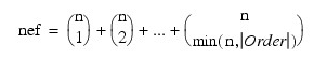
where n is given by N_ELEMENTS(n_levels) if POOL_INTER is specified; otherwise, N_ELEMENTS(N_levels) – 1.
Suppose the factors are A, B, C, and error. With ORDER = 3, rows 0 through nef – 1 correspond to A, B, C, AB, AC, BC, and ABC. The columns of TEST_EFFECTS are as follows:
- 0: Degrees of freedom
- 1: Sum of squares
- 2: F-statistic
- 3: p-value
Version History