The IMSL_LAPLACE_INV function computes the inverse Laplace transform of a complex function.
This routine requires an IDL Advanced Math and Stats license. For more information, contact your sales or technical support representative.
The IMSL_LAPLACE_INV function computes the inverse Laplace transform of a complex-valued function. Recall that if f is a function that vanishes on the negative real axis, then the Laplace transform of f is defined by:
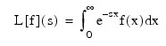
It is assumed that for some value of s the integrand is absolutely integrable.
The computation of the inverse Laplace transform is based on a modification of Weeks’ method (see Weeks (1966)) due to Garbow et al. (1988). This method is suitable when f has continuous derivatives of all orders on [0, ∞). In particular, given a complex-valued function F(s) = L[f] (s), f can be expanded in a Laguerre series whose coefficients are determined by F. This is fully described in Garbow et al. (1988) and Lyness and Giunta (1986).
The algorithm attempts to return approximations g(t) to f(t) satisfying:
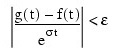
where ε = PSEUDO_ACC and σ = Sigma > sigma0. The expression on the left is called the pseudo error. An estimate of the pseudo error is available in ERR_EST.
The first step in the method is to transform F to φ where:
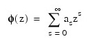
Then, if f is smooth, it is known that φ is analytic in the unit disc of the complex plane and hence has a Taylor series expansion:
which converges for all z whose absolute value is less than the radius of convergence Rc. This number is estimated in the output keyword R. Using the output keyword K, the smallest number K is estimated which satisfies:

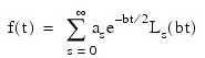
The coefficients of the Taylor series for φ can be used to expand f in a Laguerre series:
Examples
Example 1
This example computes the inverse Laplace transform of the function (s – 1)−2, and prints the computed approximation, true transform value, and difference at five points. The correct inverse transform is xex. From Abramowitz and Stegun (1964).
.RUN
FUNCTION fcn, x
one = COMPLEX(1.0, 0.0)
f = one/((x - one)*(x - 1))
RETURN, f
END
.RUN
n = 5
l_inverse = IMSL_LAPLACE_INV('fcn', 1.5, t)
relative_diff = ABS((l_inverse - true_inverse) / true_inverse)
PM, [[t(0:*)], [l_inverse(0:*)], [true_inverse(0:*)], $
[relative_diff(0:*)]], $
Title = ' t f_inv true diff'
END
t f_inv true diff
0.500000 0.824348 0.824361 1.48223e-05
1.50000 6.72247 6.72253 1.01432e-05
2.50000 30.4562 30.4562 2.50504e-07
3.50000 115.906 115.904 1.84310e-05
4.50000 405.053 405.077 5.90648e-05
Example 2
This example computes the inverse Laplace transform of e−1/s/s, and prints the computed approximation, true transform value, and difference at five points. Additionally, the inverse is returned, and a required accuracy for the inverse transform values is specified. The correct inverse transform is:
J0 (2 x)
.RUN
FUNCTION fcn, x
one = COMPLEX(1.0, 0.0)
s_inverse = one / x
f = s_inverse*EXP(-1*(s_inverse))
RETURN, f
END
.RUN
n = 5
l_inverse = IMSL_LAPLACE_INV('fcn', 0.0, t, $
Pseudo_Acc = 1.0e-6, Indicator = indicator)
true_inverse = FLOAT(IMSL_BESSJ(0, 2.0*SQRT(t)))
relative_diff = ABS((l_inverse - true_inverse) / true_inverse)
FOR i = 0, 4 DO BEGIN
IF (indicator(i) EQ 0) THEN BEGIN
PM, t(i), l_inverse(i), true_inverse(i), $
relative_diff(i), $
Title = ' t f_inv true diff'
ENDIF ELSE BEGIN
PRINT, 'Overflow or underflow noted.'
ENDELSE
ENDFOR
END
t f_inv true diff
0.500000 0.559134 0.559134 1.06602e-07
t f_inv true diff
1.50000 -0.0229669 -0.0229670 4.21725e-06
t f_inv true diff
2.50000 -0.310045 -0.310045 9.61226e-08
t f_inv true diff
3.50000 -0.401115 -0.401115 2.22896e-07
t f_inv true diff
4.50000 -0.370335 -0.370336 4.02369e-07
Syntax
Result = IMSL_LAPLACE_INV(F, Sigma0, T [, BIG_COEF_LOG=variable] [, BVALUE=parameter] [, COND_ERR=variable] [, DISC_ERR=variable] [, /DOUBLE] [, ERR_EST=variable] [, INDICATORS=variable] [, K=variable] [, MTOP=value] [, PSEUDO_ACC=value] [, R=variable] [, SIGMA=parameter] [, SMALL_COEF_LOG=variable] [, TRUNC_ERR=variable])
Return Value
A one-dimensional array containing the discrete convolution of x and x, or x and x if x
is supplied.
Arguments
F
Scalar string specifying the user-supplied function for which the inverse Laplace transform will be computed.
Sigma0
An estimate for the maximum of the real parts of the singularities of f. If unknown, set sigma0 = 0.0.
T
One-dimensional array of size n containing the points at which the inverse Laplace transform is desired.
Keywords
BIG_COEF_LOG (optional)
Named variable into which the logarithm of the largest coefficient in the decay function is stored. See the description at the beginning of this topic for details.
BVALUE (optional)
The second parameter of the Laguerre expansion. If BVALUE is less than 2.0*(Sigma − sigma0), it is reset to 2.5*(Sigma − sigma0). Default: 2.5*(Sigma − sigma0)
COND_ERR (optional)
Named variable into which the estimate of the pseudo condition error on the basis of minimal noise levels in the function values is stored.
DISC_ERR (optional)
Named variable into which the estimate of the pseudo discretization error is stored.
DOUBLE (optional)
If present and nonzero, double precision is used.
ERR_EST (optional)
Named variable into which an overall estimate of the pseudo error, DISC_EST + TRUNC_ERR + COND_ERR is stored. See the description at the beginning of this topic for details.
INDICATORS (optional)
Named variable into which an one-dimensional array of length n containing the overflow/underflow indicators for the computed approximate inverse Laplace transform is stored. Table 9-1 shows, for the i-th point at which the transform is computed, what INDICATORS(i) signifies.
|
Indicators(i) |
Meaning |
|
1 |
Normal termination.
|
|
2 |
The value of the inverse Laplace transform is too large to be representable. This component of the result is set to NaN.
|
|
3 |
The value of the inverse Laplace transform is found to be too small to be representable. This component of the result is set to
0.0. |
|
4 |
The value of the inverse Laplace transform is estimated to be too large, even before the series expansion, to be representable. This component of the result is set to NaN.
|
|
5 |
The value of the inverse Laplace transform is estimated to be too small, even before the series expansion, to be representable. This component of the result is set to 0.0.
|
K (optional)
Named variable into which the coefficient of the decay function is stored. See the description at the beginning of this topic for details.
MTOP (optional)
An upper limit on the number of coefficients to be computed in the Laguerre expansion. The keyword MTOP must be a multiple of four. Default: 1024
PSEUDO_ACC (optional)
The required absolute uniform pseudo accuracy for the coefficients and inverse Laplace transform values. Default: SQRT(ε), where ε is machine epsilon
R (optional)
Named variable into which the base of the decay function is stored. See the description at the beginning of this topic for details.
SIGMA (optional)
The first parameter of the Laguerre expansion. If SIGMA is not greater than sigma0, it is reset to sigma0+ 0.7. Default: sigma0+ 0.7
SMALL_COEF_LOG (optional)
Named variable into which the logarithm of the smallest nonzero coefficient in the decay function is stored. See the description at the beginning of this topic for details.
TRUNC_ERR (optional)
Named variable into which the estimate of the pseudo truncation error is stored.
Version History