Use the Topographic Shading Tool to blend a color representation of a digital elevation model (DEM) with a topographic feature. Examples of topographic features include shaded relief, slope, aspect, and derivatives of slope and aspect. The result is an image that provides a better visual representation of the shape and texture of topographic features than using the DEM alone. A common use is to blend a colored DEM with a shaded relief image to produce a hillshade image that emphasizes terrain relief.
You can preview the resulting image as you adjust settings for the DEM, topographic features, and the level of blending. Then you can save the result to an ENVI-format image with the same spatial resolution as the input DEM. The resulting image can be used for visualization and presentation.
You can also write a script to perform topographic shading using one of the following tasks: TopographicShadingUsingHLS, TopographicShadingUsingHSV, or TopographicShadingUsingRGB.
See the following sections:
Prepare Input Data
The Topographic Shading Tool accepts any single-band raster as input. The most common type of input is a DEM; however, you can also use the following:
- Gridded bathymetry data
- Total Magnetic Intensity (TMI) gridded data from geophysical surveys
The term DEM will be used throughout this help topic to refer to the input data you provide.
If the source raster covers a large geographic area and you are only interested in a specific region, you should create a spatial subset of that region before using the Topographic Shading Tool. This ensures that the output image will have the highest possible resolution for the area of interest.
Run the Topographic Shading Tool
- From the Toolbox, select Terrain > Topographic Shading Tool.
- In the Data Selection dialog, select a single-band DEM and click OK. The Topographic Shading Tool appears with a preview of the colored DEM blended with a shaded relief image. You can zoom in and out of the image using the scroll wheel on your mouse.
The right side of the tool is split into three sections: DEM, Topographic, and Blend. These sections are described below.
You can experiment with different DEM, Topographic, and Blend Settings; or you can select a predefined setting from the Presets drop-down list at the bottom of the tool. See Use Presets for more information.
Set DEM Parameters
Use the DEM section of the Topographic Shading Tool to modify the appearance of the DEM. You can set the stretch type, set the minimum and maximum histogram values, and modify the color table that is applied to the DEM.
- From the DEM Stretch drop-down list, select an option to stretch the DEM values within the range specified in the histogram. The options are as follows:
- Linear: Pixel values greater than the maximum histogram value are assigned a value of 255. Pixel values less than the minimum histogram value are assigned a value of 0. Pixel values between these points are linearly stretched. By distributing pixel values across the entire histogram range, the image becomes brighter and more contrasted.
- Equalization: This is a histogram equalization stretch, which scales the data to have the same number of digital numbers (DNs) in each display histogram bin.
- Gaussian: This stretch type sets the mean DEM value to a screen value of 127. It sets the data value that is three standard deviations below the mean value to a screen value of 0. Then it sets the data value that is three standard deviations above the mean value to a screen value of 255. Intermediate values are assigned screen values using a Gaussian curve.
- Square Root: ENVI calculates the square root of the input histogram and applies a linear stretch.
- Logarithmic: ENVI logarithmically stretches the gray scale of the input image. This is a non-linear technique where the low-range brightness is enhanced. The logarithmic stretch is useful for enhancing features lying in the darker parts of the original image.
- Specify the minimum and maximum histogram values for the DEM by dragging the left and right vertical sliders in the histogram. Or, type minimum and maximum values in the fields provided and press the Enter key.
Define Colors
Use the Color Table section of the Topographic Shading Tool to define the colors to apply to the DEM. Click the Edit Color Table button  . In the Edit Table Color dialog that appears, you can choose from the complete list of predefined IDL color tables, define a color gradient, or work with different color spaces. See Edit Color Tables for details.
You can also right-click on the previewed color table and choose from a list of several color tables, without having to display the Edit Color Table dialog.
Click the Reverse button  to reverse the colors in the currently selected color table.
Set Topographic Parameters
Use the Topographic section of the Topographic Shading Tool to select a topographic feature to blend with the DEM. The features are automatically created from the DEM.
-
Select a topographic feature from the drop-down list provided. The choices are as follows (see Background for details on each option):
- Slope
- Aspect
- Shaded Relief (the default)
- Profile Convexity
- Plan Convexity
- Longitudinal Convexity
- Cross Sectional Convexity
- Minimum Curvature
- Maximum Curvature
- RMS
- Slope Percent
See Background for descriptions of the options.
- Enter a Kernel Size (in pixels) used for fitting a quadratic surface to the DEM and for deriving the topographic features. The default value is 3 pixels, which represents a 3 x 3 moving window. Increasing the kernel size will smooth the results. The following figures show a comparison from the preview window:
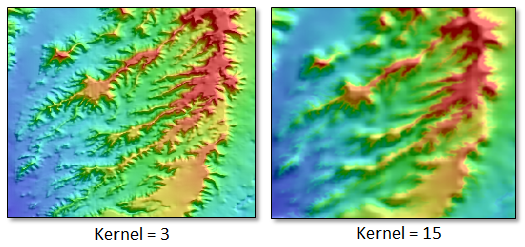
The level of smoothness in the previewed image will differ from that of the full-resolution result. The previewed image is a down-sampled version of the full-resolution image. The kernel size is directly related to the size of the full-resolution image, not the previewed image. For example, if the original image is 2400 x 2400 pixels and the previewed image is 800 x 800 pixels, a kernel size of 5 in the previewed image will be the same as a kernel size of 15 in the full-resolution image (5 times a scale factor of 3). So if you like how the kernel setting looks in the previewed image, multiply that value by a scale factor to ensure the same result in the full-resolution. Be aware, however, that increasing the kernel size significantly will increase processing time.
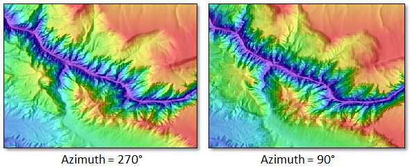
- Enter an Azimuth angle in degrees. This is the compass direction that the sun is facing, relative to geographic north. Azimuth is only used with the Shaded Relief option. Azimuth values increase in a clockwise direction from 0 degrees (north) to 360 degrees. The default value is 45 degrees. Modifying this value will affect the locations of shadows in the hillshade image, which helps to emphasize terrain features and valleys. In the following example from the preview window, an azimuth value of 270 degrees creates a more natural illusion of depth in a river gorge:
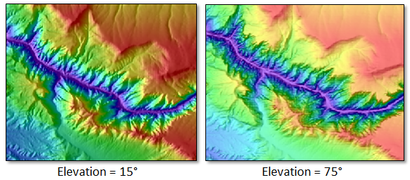
- Enter an Elevation angle in degrees. This is the sun's angle above the horizon. Elevation is only used with the Shaded Relief option. Elevation values increase from 0 degrees (the horizon) to 90 degrees (directly overhead). The default value is 55 degrees. Modifying this value will affect the brightness and shadows in the image:
- From the Topographic Stretch drop-down list, select an option to stretch the topographic feature values within the range specified in the accompanying histogram. The options are as follows:
- Linear: Pixel values greater than the maximum histogram value are assigned a value of 255. Pixel values less than the minimum histogram value are assigned a value of 0. Pixel values between these points are linearly stretched. By distributing pixel values across the entire histogram range, the image becomes brighter and more contrasted.
- Equalization: This is a histogram equalization stretch, which scales the data to have the same number of digital numbers (DNs) in each display histogram bin.
- Gaussian: This stretch type sets the mean DEM value to a screen value of 127. It sets the data value that is three standard deviations below the mean value to a screen value of 0. Then it sets the data value that is three standard deviations above the mean value to a screen value of 255. Intermediate values are assigned screen values using a Gaussian curve.
- Square Root: ENVI calculates the square root of the input histogram and applies a linear stretch.
- Logarithmic: ENVI logarithmically stretches the gray scale of the input image. This is a non-linear technique where the low-range brightness is enhanced. The logarithmic stretch is useful for enhancing features lying in the darker parts of the original image.
- Specify the minimum and maximum histogram values for the topographic feature by dragging the left and right vertical sliders in the histogram. Or, type minimum and maximum values in the fields provided and press the Enter key.
Set Blend Parameters
Use the Blend section of the Topographic Shading Tool to specify the level of blending between the DEM and topographic feature, along with the color model to use with blending.
- Select a color model. The options are as follows:
- Standard: Red/green/blue (RGB)
- HLS: Hue/lightness/saturation. The colored DEM is converted from RGB to HLS color space. Lightness and saturation are substituted with the topographic feature image. Then this combination is converted back to RGB space.
- HSV: Hue/saturation/value. The colored DEM is converted from RGB to HSV color space. Saturation and value are substituted with the topographic feature image. Then this combination is converted back to RGB space.
The HLS and HSV options add highlights to topographic features. They often give shaded relief images a glossy or metallic appearance. See the Examples section below.
Tip: Be aware that selecting a color table that contains greyscale values may produce unexpected patches of red in the output image, if you select the HLS or HSV option. An example of a greyscale value is [0, 0, 0] or [122, 122, 122]. When greyscale values are transformed to hue values, they lose their grey color and are colored red instead.
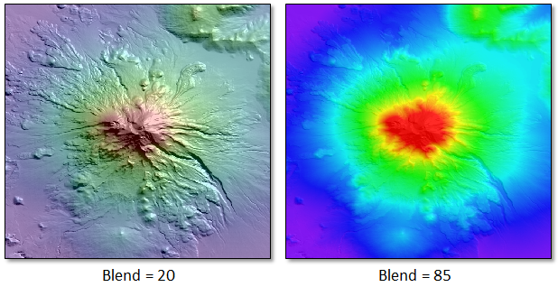
- Click and drag the Blend slider to adjust the transparency between the topographic feature image and the colored DEM. The Blend slider is only available with the Standard color model. Decreasing the Blend value will show more of the topographic feature image, while increasing the Blend value will show more of the DEM with the color table applied; for example:
Use Presets
Once you create a combination of settings that you like, you can save them as a custom preset that you can apply to other DEMs. This prevents you from having to manually set each parameter multiple times with different datasets. You can also choose from several presets by selecting them from the Presets drop-down list. The following presets are available:
- Standard: Hillshade image with a 50% blend
- Glossy-A and Glossy-B: Add highlights that give a shiny appearance
- Extreme: Hillshade image that emphasizes terrain relief instead of color
- Muted: Hillshade image that emphasizes color instead of terrain relief
- Overhead: Simulates the sun directly overhead, showing relief with no discernable direction
- Slopes: Increases brightness where slopes are highest
- Grayscale: Greyscale hillshade image with a 20% blend to show more terrain features
- Waves: Applies a Waves standard color table to give the image a contour-like appearance
- Sharp: Enhances details in terrain; best with high-quality, clean DEMs
- Smooth: Smooths terrain into a more generic shape; best with noisy DEMs
When you create your own preset, you can choose which parameters to include and the specific values they use. Parameters that you choose not to include will remain unchanged when you or another user selects that preset, allowing you to further modify those parameters. Consider what makes your preset unique, and specify only those parameters that make it unique.
Follow these steps to define and save a custom preset:
- Click the Presets drop-down list at the bottom of the tool and select Save Preset. The Save Topographic Shading Preset dialog appears.
- Select the parameters to include in the preset by selecting the Yes option. The preset will retain the currently selected values for those parameters. Select the No option for parameters that should remain unchanged.
- With DEM Stretch Max/Min and Topographic Stretch Max/Min, you can choose to save the current Min and Max values as a percentage of the total histogram or as specific values. The Percentage option is best when the preset will be used with multiple DEMs that have widely varying data ranges. The Value option is best when the preset will be used with multiple DEMs that have the same range of data values, and you want apply colors to specific data values.
- The Azimuth and Elevation options are only available when Topographic Product is set to Yes.
- Choose a filename and location for the preset file (.json).
- Click OK.
You can also restore previously saved presets by clicking Load Presets and choosing a preset file (.json). The restored preset is added to the top of the Presets list.
Create an Output Image
Once you have experimented with different settings and the previewed image looks good, you can save the result to a full-resolution RGB image in ENVI format. Follow these steps:
- Click the Apply button in the Topographic Shading tool. The Output Topographic Shading Result dialog appears.
- Select a filename and location for the output image (.dat).
- Enable the Display result check box to display the output in the view when processing is complete. Otherwise, if the check box is disabled, the result can be loaded from the Data Manager.
-
To reuse these task settings in future ENVI sessions, save them to a file. Click the down arrow next to the OK button and select Save Parameter Values, then specify the path and filename to save to. Note that some parameter types, such as rasters, vectors, and ROIs, will not be saved with the file. To apply the saved task settings, click the down arrow  and select Restore Parameter Values, then select the file where you previously stored your settings.
-
To run the process in the background, click the down arrow next to the OK button and select Run Task in the Background. If an ENVI Server has been set up on the network, the Run Task on remote ENVI Server name is also available. The ENVI Server Job Console will show the progress of the job and will provide a link to display the result when processing is complete. See ENVI Servers for more information.
- Click OK
Examples
This section provides example topographic shading images, along with the settings that were used to create them.
Shaded Relief Image of Vernal, Utah, USA
This image emphasizes the shapes and textures of anticlinal valleys and synclinal ridges near Dinosaur National Monument along the Utah-Colorado border. The selected color table also works well for creating base maps.
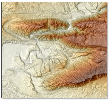
Source: U.S. Geological Survey (USGS) National Elevation Dataset (NED) DEM at 1/3-arc second resolution
DEM Stretch: Linear
Color Table: CB-YlOrBr (predefined)
Topographic Feature: Shaded Relief
Kernel: 3
Azimuth: 278
Elevation: 65
Topographic Stretch: Gaussian
Blend Settings: Standard with a Blend level of 50
Slope Image of Mount Shasta, California, USA
The brightest pixels in this image represent steeper slopes. An HLS color blending highlights the slopes better than the Standard (RGB) option would.
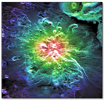
Source: USGS NED DEM at 1/3-arc second resolution
DEM Stretch: Linear
Color Table: Rainbow (predefined)
Topographic Feature: Slope
Kernel: 5
Topographic Stretch: Gaussian
Blend Settings: HLS
Shaded Relief Image Derived from Coastal LiDAR data, Mississippi, USA
The ENVI LiDAR application was used to create a DEM at 0.5-foot resolution from an unmanned aerial system (UAS) LiDAR survey. The shaded relief image was created from the DEM. It shows the terrain above and below the water surface. The HLS color space gives the shaded relief image a glossy appearance.
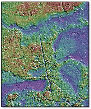
Source: NOAA Office for Coastal Management (OCM), 2017 Unmanned Aerial Systems Lidar, Grand Bay National Estuarine Research Reserve. Data available at https://coast.noaa.gov/dataviewer.
DEM Stretch: Linear
Color Table: Mac Style (predefined)
Topographic Feature: Shaded Relief
Kernel: 5
Azimuth: 45
Elevation: 55
Topographic Stretch: Gaussian
Blend Settings: HSV with the Invert Saturation option enabled
Magnetic Anomaly Image of Midwestern USA
This image is a spatial subset of a magnetic anomaly map of the continental U.S. showing the total intensity of the Earth's magnetic field after removal of the International Geomagnetic Reference Field (IGRF). The red areas show the highest anomalies, and the white areas show the lowest anomalies.
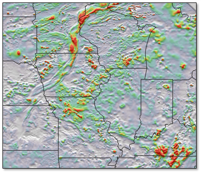
Multiple steps were taken to create this image:
- Open the original Esri GRID data in ENVI.
- Create a spatial subset of the midwestern U.S.
- Save the result to ENVI raster format.
- Run the Topographic Shading Tool using the parameters listed below.
- Display the state boundary shapefile with the resulting image.
Source: Digital data grids for the magnetic anomaly map of North America, available from the U.S. Geological Survey at https://mrdata.usgs.gov/magnetic/.
DEM Stretch: Linear
Color Table: Hue Sat Lightness 2 (predefined)
Topographic Feature: Shaded Relief
Kernel: 9
Azimuth: 0
Elevation: 70
Topographic Stretch: Linear
Blend Settings: Standard with a Blend level of 60
See Also
Topographic Modeling