In this tutorial, you will learn how to use the Spectral Angle Mapper (SAM) and Spectral Feature Fitting (SFF) methods to compare known reference spectra of geologic minerals to image pixel spectra. This will help to find pixels that are similar to the known spectra.
See the following sections:
This tutorial is one in a series of hyperspectral analysis tutorials. See the following links for additional tutorials:
Files Used in this Tutorial
Tutorial files are available from our ENVI Tutorials web page. Click the Hyperspectral link to download the .zip file to your machine, then unzip the files. You will use these files in the tutorial:
|
File |
Description |
|
CupriteReflectance.dat
|
AVIRIS reflectance image and header file
|
|
CupriteMineralROIs.xml
|
Region of interest (ROI) file with known mineral occurrences
|
You will also use some mineral spectral library files that are included with your ENVI installation.
The image used in this exercise was collected by the Airborne Visible Infrared Imaging Spectrometer (AVIRIS) sensor. AVIRIS data files are courtesy of NASA/JPL-Caltech. The sample image covers the Cuprite Hills area of southern Nevada, an area with diverse mineral types. The scene was collected from an ER-2 aircraft on August 8, 2011.
The full radiance scene is available from NASA/JPL. This image was processed as follows, resulting in the file CupriteReflectance.dat:
- Spatially subsetted
- Processed with FLAASH to remove atmospheric effects and to create a surface reflectance image in ENVI format
- 53 bands marked as "bad" in the ENVI header file. These are primarily water vapor bands that cause spikes in the reflectance curve.
- 1260 to 1560 nm (Bands 98-128)
- 1760 to 1960 nm (Bands 148-170)
See the Preprocessing AVIRIS Tutorial for the steps used to create the reflectance image.
Background
Several methods have been developed to identify ground-cover types in remote sensing imagery. Basic methods such as supervised classification produce a thematic map of the input image by measuring the similarity of image spectra to known references. Results from methods such as this are referred to as whole-pixel analysis methods because they attempt to answer the question, "Is a given material present in this image pixel?"
The Basic Hyperspectral Analysis tutorial showed how to compare image spectra to library spectra within a spectral profile plot, in attempting to identify different minerals within a scene. However, with hundreds of library spectra available, this manual process is too time-consuming. A more automated, scientifically robust method is preferred.
ENVI provides two whole-pixel analysis methods that are specially suited to hyperspectral imagery: SAM and SFF. Both are based on different principles and provide independent analyses of the same scene.
Spectral Angle Mapper (SAM)
SAM is an automated classification method for comparing image spectra to known spectra. Reference spectra, or training classes, can come from any of the following sources:
- Spectral libraries
- ASCII files
- Regions of interest (ROIs)
For the SAM classification to be effective, the input image must be converted to apparent reflectance so that the data units are the same as the library units. The image you will use in this tutorial has already been converted to apparent reflectance.
SAM determines the similarity between an image spectrum (representing an unknown material) and a reference spectrum (representing a known material) by computing the spectral angle between them, treating them as vectors in n-dimensional spectral space, where n is the number of bands.
The simplest way to illustrate this method is to create a 2D scatter plot of an image spectrum and library spectrum in a two-band image.
Here are some key points about the SAM classifier:
- Smaller angles represent closer matches to the reference spectrum.
- Pixels further away than a specified maximum angle threshold (in radians) are not classified.
- A vector from the origin through each point describes the position of each respective spectrum under all possible illumination conditions. SAM is insensitive to illumination and albedo effects, which means that all possible illuminations are treated equally.
- Poorly illuminated pixels fall closer to the origin of the scatter plot.
- The color of a material is defined by the direction of its unit vector.
- The angle between the vectors is the same, regardless of their length.
SAM generalizes this geometric relationship to n-dimensional space, where n is the number of bands in the image. For each reference spectrum chosen from hyperspectral image analysis, ENVI computes the spectral angle in radians for every image spectrum (pixel). SAM produces the following results:
Rule Images
Each rule image represents the spectral angle between the image spectrum and one reference spectrum. Darker pixels in the rule images represent smaller spectral angles and thus image spectra that are more similar to the reference spectrum. You can use the rule images for subsequent classifications using different thresholds to decide which pixels are included in the SAM classification image.
SAM Classification Image
This image assigns each pixel to a class that represents one of the materials from the selected library spectrum. The classification chooses the library spectrum that has the smallest spectral angle with each pixel in the input image. So, the classification image shows the best match to a given material for each pixel.
Spectral Feature Fitting (SFF)
SFF may be considered the first step towards a knowledge-based system for expert identification of image spectra. It is an absorption feature-based method for matching image (pixel) spectra to reference spectra. To obtain the best results from SFF classification, you need to pick the narrowest spectral range that contains the entire absorption feature. By isolating an absorption feature, you achieve the best fit with the least error.
SFF has the following requirements:
- Select the reference spectra from the image or from a spectral library.
- Remove the continuum from both the image and reference spectra prior to analysis. A continuum is a mathematical function used to isolate a given absorption feature for analysis. It corresponds to a background signal that is unrelated to the specific feature of interest.
- Scale the reference spectra to match the image spectra.
SFF goes through the following steps:
- Produces a scaled image for each endmember that you select. Endmembers are materials that are spectrally unique (or pure) within the wavelengths of a given image.
- Subtracts the continuum-removed spectra from 1.0, thus inverting it and making the continuum zero.
- Determines a single multiplicative scale factor that matches the reference spectrum to the pixel spectrum. Assuming that you selected an accurate absorption feature wavelength range, a large scale factor indicates a deep spectral feature.
- Performs a band-by-band, least-squares fit between each reference spectrum and the pixel spectra.
- Produces a root mean squared (RMS) image for each reference spectrum.
Exercise 1: SAM Classification
This exercise shows how to use SAM to classify different minerals in an AVIRIS image. For training data, you will import a region of interest (ROI) file of known mineral types in this image.
Open AVIRIS Image and Mineral ROIs
- Start ENVI.
- Click the Open button
 in the toolbar.
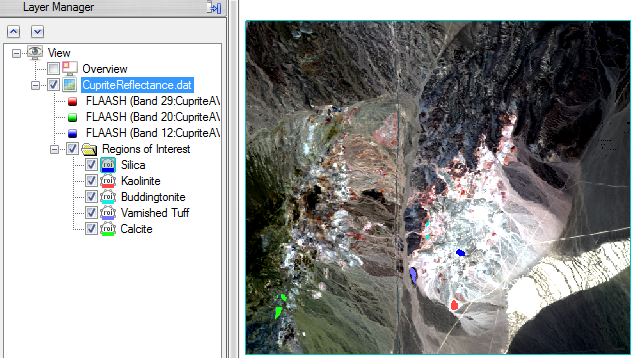
- Select the file CupriteReflectance.dat and click Open. Out of the 224 bands of this AVIRIS scene, ENVI automatically determines the best bands to approximate a true-color display. In this case, it assigns Band 29 to red, Band 20 to green, and Band 12 to blue.
- Click the Open button in the toolbar.
- Select the ROI file CupriteMineralROIs.xml and click Open. The ROIs for each mineral are listed in the Layer Manager and displayed on top of the image.
Start SAM Classification
- In the search field of the Toolbox, type spectral angle.
- Double-click the Spectral Angle Mapper Classification tool name that appears.
- In the Classification Input File dialog, select CupriteReflectance.dat but do not click OK yet.
- Click the Spectral Subset button.
- Click the Clear button to clear the selection list.
- In this step, you will select bands that encompass characteristic absorption features of minerals in the range of 1998 to 2437 nanometers. Click Band 174, hold down the Shift key on your keyboard, and click Band 218.
- Click the Add Range button, then OK in both the File Spectral Subset dialog and the Classification Input File dialog.
Define Training Data
- The Endmember Collection dialog is used for any classification and mapping tool that requires you to specify reference spectra. Using the Algorithm menu, you can apply any classification method to the selected image and reference spectra. Notice that Spectral Angle Mapper is the selected method under the Algorithm menu.
- From the Endmember Collection dialog menu bar, select Import > from ROI/EVF from input file. The next dialog lists the individual ROIs that are available.
- For this exercise, you will just analyze two minerals. Use the Ctrl key on your keyboard to select Buddingtonite and Kaolinite, then click OK.
- Click the Select All button in the Endmember Collection dialog, then click Apply.
Define SAM Parameters
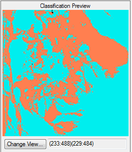
- In the Spectral Angle Mapper Parameters dialog, you can preview the initial classification before continuing. Click the Preview button.
- The preview is restricted to a 256 x 256 pixel bounding box. Follow these steps to change the location of the bounding box:
- Click the Change View button underneath the preview.
- Click the Image button in the Select Spatial Subset dialog.
- Move the red bounding box to a different location.
- Click OK in the Subset by Image dialog, then again in the Select Spatial Subset dialog.
The preview updates to show the new location. Notice that the initial classification image is comprised entirely of the buddingtonite and kaolinite classes, as the following example shows. This is not accurate, so you need to lower the spectral angle so that the SAM classification is more restrictive.
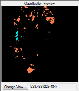
- In the Spectral Angle Mapper Parameters dialog, change the Maximum Angle (radians) value to 0.04.
- Click Preview. Now more pixels are unclassified (black), leaving the buddingtonite and kaolinite classes with fewer pixels:
- Experiment with a different value to apply to both classes (using the Single Value button), or click Multiple Values and assign different maximum angle values to each class.
- In the center part of the Spectral Angle Mapper Parameters dialog, enter the filename CupriteSAMClass.dat for the SAM classification image.
- Leave the default selection of Yes for Output Rule Images?, then enter the filename CupriteSAMRule.dat for the rule file.
- Click OK to start the classification. When processing is complete, the Layer Manager lists the classification image and buddingtonite rule image. The classification image appears in the display.
- Close the Endmember Collection dialog.
View Rule Images
Rule images are helpful in interpreting classification data. For the SAM classifier, rule images show the similarity between the image pixel's spectrum and the reference spectra from training data. Darker pixels in the rule images represent smaller spectral angles and thus image spectra that are more similar to the reference spectrum.
The rule file that you just created (CupriteSAMRule.dat) contains two bands: one each for the buddingtonite and kaolinite rule images. ENVI only lists one band in the Layer Manager (buddingtonite).
- Before you view the rule images, use the check boxes to turn off the following layers in the Layer Manager:
- Unclassified and Buddingtonite classes, under the Classes folder of CupriteSAMClass
- CupriteReflectance.dat
- Regions of Interest
- Click the Data Manager button
 in the toolbar. Scroll to the bottom of the file list until you see CupriteSAMRule.
- Select Rule (Kaolinite) and click the Load Grayscale button. The kaolinite rule image appears in the display.
- Select the CupriteSAMClass layer in the Layer Manager, and drag it above the layer that contains the kaolinite rule image. The kaolinite class from the SAM classification image displays on top of the kaolinite rule image. The following figure shows an example:
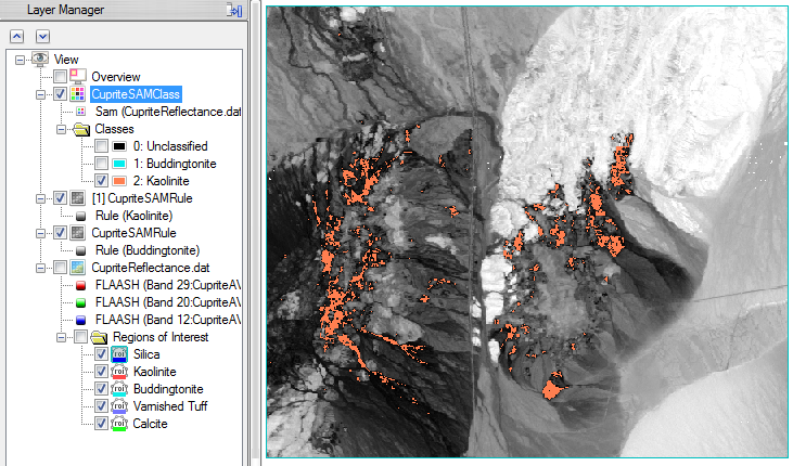
- Toggle the Kaolinite class on and off, to compare the classification results against the rule image. The darkest pixels in the rule image represent the closest matches to the ROI training data, in terms of spectral angle.
- Repeat the previous two steps for the Buddingtonite class. Compare the classification results against the buddingtonite rule image.
- To prepare for the next exercise, open the Data Manager and close all files except for CupriteReflectance.dat.
Exercise 2: Spectral Feature Fitting
Spectral Feature Fitting (SFF) compares a specific absorption feature from each image pixel to that of a known reference spectrum. Pixels whose absorption feature spectra match well in width and depth are likely to have a higher abundance of the material of interest. SFF works best with materials that have unique and detailed absorption features such as minerals and some man-made features. In contrast, it does not work well with general categories of materials such as vegetation and water. The reference spectra for this exercise come from spectral libraries of minerals.
In this exercise, you will remove the continuum spectrum from the AVIRIS scene, plot a library spectrum of the mineral alunite, then create SFF scale and RMS images that show how well the image spectra match the absorption feature of the library spectrum.
Remove the Continuum
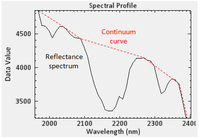
SFF requires you to first remove the continuum from the image and reference spectra. Removing the continuum normalizes each spectrum in the input reflectance image by comparing it to a continuum curve, thus defining a common baseline from which to measure absorption feature depth and position. A continuum curve is a mathematical function formed by fitting a convex hull to the spectrum:
Remove the continuum by dividing it into the original spectrum. The general shape of the spectrum is removed, leaving only the absorption features. The continuum-removed image spectra are equal to 1 where the continuum and the spectra match. They are less than 1 where absorption features occur. The continuum-removed data are scaled so that pixel values are between 0 and 1. Darker areas in the continuum-removed image have larger absorption features than lighter areas.
- In the search field of the Toolbox, type contin.
- Double-click the Continuum Removal tool name that appears.
- In the Continuum Removal Input File dialog, select CupriteReflectance.dat and click OK.
- In the Continuum Removal Parameters dialog, enter an output filename of CupriteReflectanceCR.dat and click OK.
- When processing is complete, right-click on the CupriteReflectanceCR.dat layer in the Layer Manager and select Profiles > Spectral.
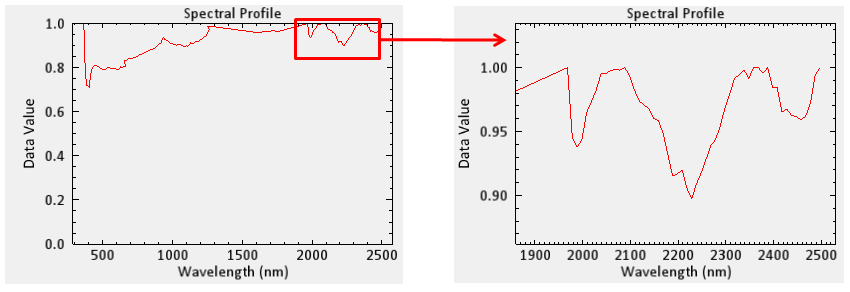
- Zoom into the wavelength range of 2000 to 2400 nm. The following example shows the spectrum from pixel location (391, 307). If your mouse has a scroll wheel, click inside the plot window and roll the wheel to zoom in. Or, click-and-drag the scroll wheel to draw a box around the area you want to zoom into. Notice how the absorption features are enhanced by removing the continuum from the image spectrum:
Collect Reference Spectra
The reference spectra you will use come from spectral libraries. Included with your installation of ENVI are several groups of library spectra from the NASA Jet Propulsion Laboratory (JPL), Johns Hopkins University (JHU), and the U.S. Geological Survey (USGS).
These library files are courtesy of the Jet Propulsion Laboratory, California Institute of Technology, Pasadena, California. Copyright © 1999, California Institute of Technology. All Rights Reserved.
- From the ENVI menu bar, select Display > Spectral Library Viewer.
- On the left side of the Spectral Library Viewer, expand the usgs (1994) folder.
- Expand the minerals_asd_2151.sli collection.
- Select the Alunite HS295 spectrum.
Run Spectral Feature Fitting
- In the search window of the toolbox, type spectral feature.
- Double-click the Spectral Feature Fitting tool name that appears.
- Select the input file CupriteReflectanceCR.dat, but do not click OK yet.
- Click the Spectral Subset button.
- Click the Clear button.
- You will obtain best results from SFF if you narrow the spectral range to include only one absorption feature of interest. In this step, you will select bands that encompass the characteristic absorption feature from 2000 to 2250 nanometers. Click Band 174, hold down the Shift key on your keyboard, and click Band 200.
- Click OK in the Spectral Feature Fitting Input File dialog.
- In this step, you will import reference spectra from the spectral library. From the Endmember Collection dialog menu bar, select Import > from Plot Windows.
- In the Import from Plot Windows dialog, click Select All Items, then OK.
- Click Apply in the Endmember Collection dialog.
- In the Spectral Feature Fitting Parameters dialog, the toggle button is set to Output separate Scale and RMS Images, which is correct for this exercise. With this option, ENVI creates a Scale and RMS image for each spectral endmember.
- Enter an output filename of CupriteSFF.dat, then click OK.
- Close the Spectral Library Viewer and Endmember Collection dialogs.
View Scale and RMS Images
- Uncheck all layers in the Layer Manager.
- From the ENVI menu bar, select Views > Two Vertical Views.
- Click the Data Manager button in the toolbar. Scroll to the bottom of the file list until you see CupriteSFF.dat.
- Drag and drop the Scale band name into the left view.
- Drag and drop the RMS band name into the right view.
- From the menu bar, select Views > Link Views. You will create a geographic link between the views.
- The Geo Link option is already selected in the Link Views dialog. Click the Link All button, then OK. Now when you pan around one view, the other view pans accordingly.
Bright areas in the Scale image indicates pixels whose absorption features are similar in depth and width to those of the alunite library spectrum. Dark areas in the RMS image indicate low RMS errors. A better analysis technique is to compare the Scale image against the RMS image. You have two options for this: (1) create a band-ratio image of the Scale and RMS images, and (2) create a scatter plot between the Scale and RMS images. For this exercise, you will create a scatter plot to look for areas where the spectral fit is good.
Create a Scatter Plot of Scale vs. RMS Image
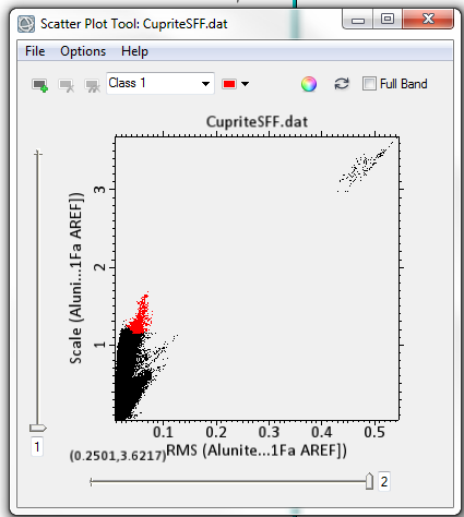
- From the menu bar, select Display > 2D Scatter Plot. In the Scatter Plot Tool dialog, note that the RMS band is assigned to the x-axis. The Scale band is assigned to the y-axis.
- Draw a polygon around a group of pixels where the RMS values are low and the Scale values are high. You can click repeatedly to define segments of a polygon, or hold down the left mouse button to draw a continuous polygon. Right-click to accept the polygon. Pixels in the image that correspond to the scatter plot points are highlighted in red. These pixels have a good spectral fit for the alunite absorption feature. The following figure shows an example.
SAM and SFF are two examples of whole-pixel analysis methods used to determine the abundance of materials of interest in a scene. For a more complex analysis, you can experiment with ENVI's Multi-Range SFF tool, in which you define multiple wavelength ranges for SFF comparison.
References
Baldridge, A., S. Hook, C. Grove, and G. Rivera. The ASTER Spectral Library Version 2.0. Remote Sensing of Environment 113 (2009): 711-715.
Clark, R., G. Swayze, and A. Gallagher, "Mapping Minerals with Imaging Spectroscopy" U.S. Geological Survey, Office of Mineral Resources Bulletin 2039 (1993): 141-150.
Kruse, F., et al. "The Spectral Image Processing System (SIPS) - Interactive Visualization and Analysis of Imaging Spectrometer Data." Remote Sensing of Environment 44 (1993): 145 - 163.