Example-Based Classification

Feature Extraction with Example Based Classification Tutorial

Example-based, or supervised, classification is the process of using training data to assign objects of unknown identity to one or more known features. The more features and training samples you select, the better the results from supervised classification.

You must have an ENVI Feature Extraction license in order to use this tool.

See the following sections:

Select Input Files for Feature Extraction
Segment Images
Select Training Data
Save Training Data
Import Ground Truth Data
Select Attributes for Classification
Select a Classification Method (Advanced)
Export Classification Results

From the Toolbox, select Feature Extraction > Example Based > Feature Extraction Workflow. The Data Selection panel appears.

Select Input Files for Feature Extraction

For best results with Feature Extraction, consider preprocessing your imagery to reduce noisy or redundant data, to correct for atmospheric effects, or to suppress vegetation. See Preprocess Imagery for available options.

For hyperspectral imagery, we strongly recommend that you run a principal components analysis or independent components analysis on the dataset before using it in Feature Extraction. Segmentation and merging work best on datasets with only a few bands.

Also consider reducing the spatial resolution of your input image to speed up processing and to remove small, unwanted features. For example, you can down-sample a 10,000 by 10,000 pixel image by a factor of 10 to yield a 1,000 by 1,000 pixel image.

Click Browse and select a panchromatic or multispectral image for input using the Data Selection dialog. Feature Extraction accepts any image format listed in Supported Data Types.
To apply a mask, select the Input Mask tab in the File Selection panel. In addition to the mask, any pixel values specified in the Data Ignore Value field of the associated header (for ENVI-format files) will be treated as mask values and will not be processed by Feature Extraction.
You can import ancillary data to help extract features of interest. An example is combining a LiDAR digital surface model (DSM) with a multispectral image to identify rooftops in a residential area, then building a rule using height data from the DSM to more accurately extract the rooftops. (The height data would be in the Spectral Mean attribute for the DSM band.) Multiple datasets often provide more accurate results. The following rules apply:
- You can only use raster data for ancillary data. Vector data must be converted to raster format prior to import.
- The ancillary image file must be georeferenced to a standard or Rational Polynomial Coefficient (RPC) spatial reference. If the ancillary data is not in the same map projection as the input image, ENVI will reproject the ancillary data to match the base projection. Images with a pseudo spatial reference cannot be used as ancillary data.
- The ancillary data and input image must have some geographic overlap.
- If you spatially subset the input image, the ancillary data will be reprojected to match that spatial extent.

Select the Ancillary Data tab and click Add Data. Select one or more ancillary files for input. You can select spectral subsets from each ancillary data file. ENVI will create new bands for each ancillary file that you import; you can then use these bands for rule-based classification. The ancillary bands are identified by the name of the ancillary file and the respective band number of that file.

Select the Custom Bands tab and enable the following options if desired. The input image must be georeferenced to a standard map projection for these options to be available.
- Normalized Difference: Select two bands for computing a normalized band ratio as follows:
- Color Space: Select the Red, Green, and Blue band names from the image. ENVI will perform an RGB to HSI color space transformation and will create new bands for Hue, Saturation, and Intensity that you can use for segmentation or rule-based classification.

Note: You should not perform segmentation with a combination of custom bands (normalized difference or HSI color space) and visible/NIR bands. You can perform segmentation on the normalized difference or color space bands by themselves, but not in combination with visible and NIR bands.

Click Next.

ENVI will create a single dataset from the combined bands of the input image, ancillary data, normalized difference, hue, saturation, and intensity (if selected). This single dataset will be used throughout the rest of the Feature Extraction workflow.

When file selection is complete, the file opens in a new workflow view. If the selected file is displayed in an active view before you start the workflow, the display bands and image location are retained, as well as any brightness, contrast, stretch, and sharpen settings. The image location is not retained for pixel-based images or those with pseudo or arbitrary projections.

Segment Images

Segmentation is the process of partitioning an image into objects by grouping neighboring pixels with common values. The objects in the image ideally correspond to real-world features. Effective segmentation ensures that classification results are more accurate.

Enable the Preview option in the Object Creation panel. A Preview Window appears with segments outlined in green.
Under Segment Settings, select an Algorithm from the drop-down list provided. The following options are available:
- Edge: Best for detecting edges of features where objects of interest have sharp edges. Set an appropriate Scale Level and Merge Level (see steps below) to effectively delineate features.
- Intensity: Best for segmenting images with subtle gradients such as digital elevation models (DEMs) or images of electromagnetic fields. When selecting this method, don't perform any merging; set the Merge Level to 0. Merging is used primarily to combine segments with similar spectral information. Elevation and other related attributes are not appropriate for merging.

See Watershed Algorithm Background for more detailed descriptions of each option.

Adjust the Scale Level slider as needed to effectively delineate the boundaries of features as much as possible without over-segmenting the features. Increasing the slider results in fewer segments; decreasing the slider results in more segments. You should also ensure that features of interest are not grouped into segments represented by other features. See Watershed Algorithm Background for a more detailed discussion of how the Scale Level is used with respect to gradient and intensity images.
Click the Select Segment Bands button to choose specific bands for applying the segmentation settings. The settings will apply to a grayscale image derived from the average of all selected bands. All available bands are selected by default.

Tip: For best segmentation results, select a combination of bands that have similar spectral ranges such as R, G, B, and NIR bands. You should not perform segmentation with a combination of custom bands (normalized difference or HSI color space) and visible/NIR bands. You can perform segmentation on the normalized difference or color space bands by themselves, but not in combination with visible and NIR bands.

Merging combines adjacent segments with similar spectral attributes. Under Merge Settings, select an Algorithm from the drop-down list provided. The following options are available:
- Full Lambda Schedule: (default). Merges small segments within larger, textured areas such as trees or clouds, where over-segmentation may be a problem.
- Fast Lambda: Merges adjacent segments with similar colors and border sizes.

See Merge Algorithms Background for more detailed descriptions of each option.

Adjust the Merge Level slider as needed to combine segments with similar colors (Fast Lambda) or to merge over-segmented areas (Full Lambda Schedule). Increasing the slider results in more merging; no merging will occur if you leave the slider value at 0. For example, if a red building consists of three segments, selecting Fast Lambda and increasing the Merge Level should combine them into one segment. All available bands are selected by default. To delineate treetops or other highly textured features, select Full Lambda Schedule and increase the Merge Level value.
Click the Select Merge Bands button to choose specific bands for applying the merge settings. Merging will be based on the differences between region colors based on all selected bands.
Select a Texture Kernel Size value, which is the size (in pixels) of a moving box centered over each pixel in the image. Texture attributes are computed for each kernel. Enter an odd number of 3 or higher. The maximum value is 19. The default value is 3. Select a higher kernel size if you are segmenting large areas with little texture variance such as fields. Select a lower kernel size if you are segmenting smaller areas with higher variance such as urban neighborhoods.
Click Next. ENVI loads a segmentation image into the display.

Select Training Data

The Example-Based Classification panel contains a folder called All Classes that will contain all of the feature types (classes) that you define. A new, undefined class is available for you to start defining training data.

Select the new class, and edit its name and color within the Class Properties table.
As you move around the segmentation image, the regions underneath your cursor are highlighted in cyan. Click on a highlighted region to assign it to that class. The color of the region changes to the feature color, and the class name updates to show the number of training regions you added.

Tip: Suppose you created a new class called "Vegetation." Move your cursor around the image and highlight a region that you know represents vegetation. Click on the region to select it. To view the original image instead of the segmentation image, set the Transparency slider in the main toolbar to 100% transparency.

The color variations of the segments in the segmentation image may be so small that you cannot discern them. Enable the Show Boundaries option to outline the segments so they are easier to visualize.

Continue selecting training regions that best represent your class. Try to select regions with different textures, shades, and sizes.

Another way to select training regions is to draw a box around a group of adjacent segments; however selecting a large number of segments could result in slower processing.

To remove an individual region from selection, click on it again.
To assign a training region to a different class, first select the class that you want to assign it to. Then select the training region. It changes color to reflect the newly assigned class.
To create a new class, select the class name and click the Add Class button.
To delete a class, select the class name and click the Remove Class button.

Save Training Data

To save your training data for all classes to a point shapefile, click the Save Example File button. ENVI saves the pixel coordinates of the points where you clicked when selecting training regions, along with map coordinates if the image is georeferenced.

A training data shapefile only contains the locations of training regions; it does not include other parameters you selected for example-based classification such as the classification method, selected attributes, etc.

You can later restore the training data file by clicking the Restore Example File button. The restored data will overwrite any training data you have defined in the curent session. You cannot restore a pixel-based training data file for use with a georeferenced image. After restoring the file, you can click Back to readjust your segmentation settings if needed, but the training regions will change based on the new segmentation result.

Import Ground Truth Data

Ground truth data defines areas of an image with known feature types, thus it represents a true classification for specific areas of the image. You can import ground truth data from the following sources when performing supervised classification:

Point and polygon shapefiles.
3D point and polygon shapefiles.

Tip: An example of ground truth data is a land-cover classification shapefile or geological map of your area of interest, which may be available from websites of local government agencies.

Under the Examples Selection tab, click the Import Ground Truth button. This button is enabled for georeferenced input images only.
Importing a ground truth file will overwrite any existing training samples that you have collected. When prompted to disregard the currently loaded example file, click Yes. The Data Selection dialog appears.
Click Open File and select a 2D or 3D point or polygon shapefile with ground truth data. Click OK. The Select Attribute dialog appears.
From the Select Attribute drop-down list, select the shapefile attribute to group vector records into training classes. The default is CLASS_ID. You should choose unambiguous attribute fields for grouping records into training classes.
Regions in the segmentation image that overlap any vector records in the shapefile will become training samples for the corresponding class. Vector records that do not overlap the input image will be ignored. If you select Use Centroid, a region will become a training region only if the centroid of the polygon (instead of any part of the polygon) falls within the region. A centroid is the geometric center of a polygon.
Click Import. A new class will be created for each unique CLASS_ID or other attribute value that you choose.

Define Class Colors

You can specify class colors by adding a CLASS_CLRS attribute to the ground truth shapefile. Use this attribute field to specify class colors using a string of RGB values (for example, enter '255,0,0' for Red). If the shapefile contains CLASS_NAME and CLASS_CLRS attributes and you select the CLASS_ID attribute from the Select Attribute drop-down list, the proper class names and colors will be restored. If the shapefile does not contain CLASS_NAME and CLASS_CLRS attributes, ENVI will assign unique names and colors to each class. You can rename them in the Example-Based Classification panel if desired.

Define Multiple Classes from One Shapefile

You can use a single 2D or 3D polygon shapefile to define multiple classes. An example is using the Classification workflow to draw polygons in an image that represent different classes, then saving the polygons to a shapefile:

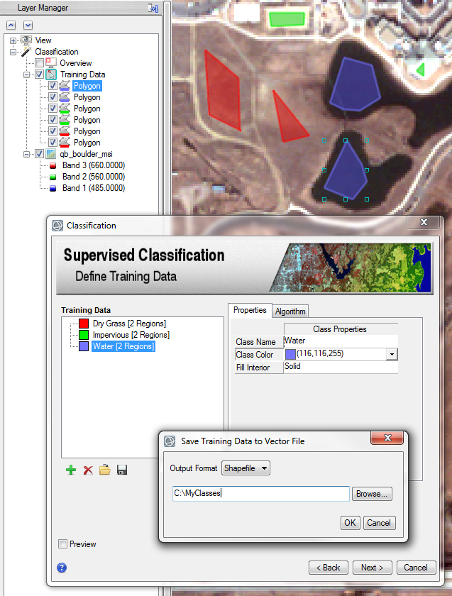
In this case, the shapefile will contain a CLASS_ID attribute with the values of each class:

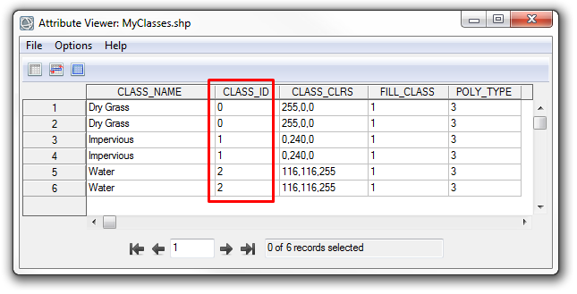
Import this shapefile as training data into the Example-Based Feature Extraction workflow using the steps above.

You do not have to use the Classification workflow to create a training data shapefile; it can come from any source as long as it has a CLASS_ID attribute defined. You can add or edit classes in the CLASS_ID field as needed. For example, suppose that you defined some regions of interest (ROIs) with several hundred polygons representing training regions, but you only want 10 classes. Export the ROIs to a shapefile, open the shapefile in ENVI, open the Attribute Viewer, and group the polygon ROIs into 10 classes by editing the CLASS_ID values. Then import the shapefile as training data in the Example-Based Classification workflow.

Select Attributes for Classification

This section describes how to choose attributes that will be used to classify your training samples. Click the Attributes Selection tab to see the available options. By default, all attributes will be used for classification.

Note: This section is disabled for PCA classification since all attributes are used with that method.

The Available Attributes column shows the attributes that are available for you to choose from. See List of Attributes for their definitions. Expand the Spatial, Spectral, and Texture groups to see individual attributes.
The Selected Attributes column shows the attributes that will be used in classification. By default, all spatial, spectral, and texture attributes are initially included. You cannot proceed with example-based classification until you select at least one attribute for classification.
To remove one or more attributes from the Selected Attributes column, select the attribute name(s) and click the < button.
To add an individual attribute back to the Selected Attributes column, select the attribute name(s) in the Available Attributes column and click the > button.
To add groups of attributes to the Selected Attributes column, select Spatial, Spectral, or Texture in the Available Attributes column, and click the > button.

To perform classification with only a few attributes (instead of all of them), select the Selected Attributes folder in the right column and click the < button. Then under the Available Attributes column, select the few attributes you want to use for classification and click the > button.
Spectral and texture attributes are computed for each band of your image. When selecting spectral and texture attributes for classification, select the specific bands to include by using the check boxes provided. Or use the Select All or Deselect all button. You can also remove a specific band by selecting it under the Selected Attributes column and unchecking it in the band list.
Click Auto Select Attributes to have ENVI determine the best attributes to use for classifying features. The underlying logic is based on the reference below. This button is enabled once you define at least two classes with at least two training samples each. The more classes and training samples you have, the slower the process.

Reference

An interval based attribute ranking technique. Unpublished report, NV5 Geospatial Solutions, Inc.. A copy of this paper is available from Technical Support.

Select a Classification Method (Advanced)

Three methods are available to perform supervised classification. Click the Algorithms tab and select a method from the Algorithms drop-down list. See one of the following sections:

KNN: This method classifies segments based on their proximity to neighboring training regions. See Background on K Nearest Neighbor for more information. The KNN method is slower compared to PCA, particularly when your segmentation image has thousands of segments. However, it is a more rigorous method that more accurately distinguishes between similar classes. You only need to define one class in order to proceed with KNN classification.
PCA: This method assigns segments to classes using a principal components analysis. You must define at least two classes with a minimum of two training regions each. See Background on Principal Components Analysis for more information.
SVM: This is the most rigorous of the three classification methods, so processing time will be slower. See Support Vector Machine Background for Feature Extraction for more information. Each class must have at least two training samples; otherwise, the class will be excluded from classification.

Enable the Allow Unclassified option to allow segments to be unclassified when the classifier cannot determine suitable classes for them. This option is enabled by default.

After the KNN, PCA, or SVM method runs, each segment is assigned the class with the highest class confidence value. Segments with class confidence values less than the percentage you set with the Threshold slider are assigned to "unclassified." The default Threshold value is 5 percent, which means segments that have less than 5 percent confidence in each class are set to "unclassified."

As you increase the Threshold slider, the classifier will allow more unclassified segments. As you decrease the value of the Threshold slider, the classifier forces more segments into classes. A value of 0 means that all segments will be classified, except with the PCA method where some unclassified regions may remain.

Enable the Preview option to view classification results within a Preview Window. You can preview the effects of changing classification options before classifying the entire image. If either the image lines or samples is greater than 1024 pixels and you want to zoom out of the data, you cannot zoom out further than 50% because it will significantly increase processing time and delay the previewed data from displaying. Zooming out further than 50% will result in a black Preview Window.

Export Classification Results

In this step, you will select the types of images, vectors, and statistics to export to various formats. By default, files are saved to the directory that you specify in the Output Directory preference. When the export is complete, the workflow view closes. The original data and the export data display in the Image window view. The available output options vary, depending on your workflow.

Rule-Based and Example-Based Classification
Segment-Only

Rule-Based and Example-Based Classification

Choose the classification file types you want to save.

Export Vector Tab

Export Classification Vectors: Save all classes to a single shapefile with a filename of <prefix>_vectors.shp. Shapefiles have a maximum file size of 2 GB, so if the image has a large number of classes and the resulting shapefile exceeds this file size, it will be broken into smaller shapefiles. Shapefiles larger than 1.5 GB cannot be displayed. To avoid these issues when working with large datasets, you can save the vectors to a geodatabase.
Merge Adjacent Features: Select this option if you are confident that adjacent polygons belong to the same class and you want to consolidate them into a single polygon. This results in a smaller file size. This option merges all adjacent segments at once across the entire image; you cannot select specific polygons to merge.

Tip: A good example is an angled rooftop that reveals different brightness levels from an aerial sensor, depending on the sun's angle. The segmentation step would typically create multiple regions within the rooftop, each with different spectral values. But if you build a good rule set that identifies rooftops, the classification image (and/or shapefile) will assign these regions to the same class. Since you know that they all belong to one rooftop, you can choose to merge the adjacent segments so that the entire rooftop is one polygon.

Export Attributes: Select this option if you want to include the spatial, spectral, and texture attributes that were computed for each region in the output shapefile.

Export Raster Tab

Export Classification Image: Create an image in ENVI raster format whose pixel values represent different classes. The filename will be <prefix>_class.dat.
Export Segmentation Image: Create a multispectral image in ENVI raster format that shows the regions defined by segmentation; each region is assigned the mean spectral values of all the pixels that belong to that region. The filename will be <prefix>_segmentation.dat.

Advanced Export Tab

Export Attributes Image: Create a multi-layer image in ENVI raster format where each layer represents the values of a specific attribute. The filename will be <prefix>_attributes.dat. When you select this option, a new dialog appears that lets you select which attributes to export to an attribute image. The Selected Attributes column is initially populated with the attributes you used in your rule set. If an attribute does not contain any valid values, then that attribute band will be assigned pixel values of 0. See Selecting Attributes for Classification for further details on using this dialog.
Export Confidence Image: Create an image in ENVI raster format that shows the relative confidence of each object belonging to a class. The higher the brightness of an object, the higher the confidence that the object belongs to the class. If an object is very dark, it likely does not belong to the class. This is a multi-layer file, with each layer representing one class. The filename will be <prefix>_confidence.dat.

Auxiliary Export Tab

Export Feature Examples: Example-based classification only. Save the training samples that you selected for all classes to an XML file named <prefix>_trainingset.ftr.
Export Feature Ruleset: Rule-based classification only. Save the rules that you defined to a file named <prefix>_ruleset.rul.
Export Processing Report: Create a text report that summarizes the segmentation options, rules, and attributes that you used to classify the image. The filename will be <prefix>_report.txt.

Segment-Only

Export Vector Tab

Export Segmentation Vectors: Save the regions in the segmentation image to a shapefile. Shapefiles have a maximum file size of 2 GB, so if your image has a large number of segments and the resulting shapefile exceeds this file size, it will be broken into smaller shapefiles. Shapefiles larger than 1.5 GB cannot be displayed.

Export Attributes: Select this option if you want to include the spatial, spectral, and texture attributes that were computed for each region in the output shapefile.

Export Raster Tab

Export Segmentation Image: Create a multispectral image in ENVI raster format that shows the regions defined by segmentation; each region is assigned the mean spectral values of all the pixels that belong to that region.

Advanced Export Tab

Export Attributes Image: Create a multi-layer image in ENVI raster format where each layer represents the values of a specific attribute. When you select this option, a new dialog appears that lets you select which attributes to export to an attribute image. The Selected Attributes column is initially empty. Select the attribute name(s) that you want to export in the Available Attributes column, and click the Add Selected Attribute button. If an attribute does not contain any valid values, then that attribute band will be assigned pixel values of 0. See Selecting Attributes for Classification for further details on using this dialog.

Auxiliary Export Tab

Export Processing Report: Create a report that summarizes the segmentation options, rules, and attributes that you used to classify the image.

Module	ENVI FX

Version	6.0