In this tutorial you will use the ENVI Modeler to build a time series of vegetation index images created from Sentinel-2 imagery. The model performs atmospheric correction and scaling of pixel values to yield surface reflectance data. The model computes a vegetation index for each input image and creates a time series from the images. You will learn how to view a time series profile and use an ISODATA classification of vegetation index values to study trends in crop health over a two-year period.
The ENVI Atmospheric Correction Module is required to use the QUick Atmospheric Correction (QUAC®) task in the ENVI Modeler.
See the following sections:
Files Used in This Tutorial
Tutorial files are available from our ENVI Tutorials web page. Click the Sentinel-2 Time Series link to download the .zip file to your machine, then unzip the files.
Twenty-three files are provided that contain Sentinel-2, Level-1C image subsets from November 18, 2018 through November 27, 2020:
|
File |
File |
|
Sentinel2_CA_2018-11-18.dat
|
Sentinel2_CA_2019-11-18.dat
|
|
Sentinel2_CA_2018-12-13.dat
|
Sentinel2_CA_2020-01-12.dat
|
|
Sentinel2_CA_2019-01-02.dat
|
Sentinel2_CA_2020-02-16.dat
|
|
Sentinel2_CA_2019-02-11.dat
|
Sentinel2_CA_2020-03-22.dat
|
|
Sentinel2_CA_2019-03-18.dat
|
Sentinel2_CA_2019-11-18.dat
|
|
Sentinel2_CA_2019-04-07.dat
|
Sentinel2_CA_2020-05-01.dat
|
|
Sentinel2_CA_2019-05-12.dat
|
Sentinel2_CA_2020-06-10.dat
|
|
Sentinel2_CA_2019-06-16.dat
|
Sentinel2_CA_2020-06-30.dat
|
|
Sentinel2_CA_2019-07-21.dat
|
Sentinel2_CA_2020-08-09.dat
|
|
Sentinel2_CA_2019-08-20.dat
|
Sentinel2_CA_2020-09-13.dat
|
|
Sentinel2_CA_2019-09-14.dat
|
Sentinel2_CA_2020-10-28.dat
|
|
Sentinel2_CA_2019-10-24.dat
|
Sentinel2_CA_2020-11-27.dat
|
The images were acquired approximately one month apart. The following steps were taken to prepare the original data files and reduce their file sizes for this tutorial:
- Built a layer stack of input 10-meter and 20-meter bands, with the 20-meter bands up-sampled to 10 meters. Each image has 10 bands: B2/blue, B3/green, B4/red, B8/near-infrared (NIR), B5/vegetation red edge, B6/vegetation red edge, B7/vegetation red edge, B8A/narrow NIR, B11/SWIR, B12/SWIR.
- Regridded and spatially subetted each image to a common projection (UTM Zone 11N, WGS-84) and spatial extent. The size of each image is 765 x 835 pixels at 10-meter spatial resolution.
See the Earth Resources Observation and Science (EROS) Center web site for more information about the USGS distribution of Sentinel-2 products, including the data policy and citation.
In addition to the 23 images, a sample model (Build Time Series.model) is provided that you will use later in the tutorial. Be sure to copy this file to your local drive as well.
Background
The goal of this tutorial is to analyze trends in crop health over a two-year period, using monthly processed satellite images. A time series of vegetation index images can reveal changes in crop health over a large geographic area or within specific fields.
For this tutorial, a random location was chosen that consisted entirely of agricultural fields. The study area is in Tulare County, California, USA. It is located in the San Joaquin Valley, which is a rich agricultural region. Crops consist of grapes, cotton, almonds, pistachios, citrus, and vegetables.
According to the United States Drought Monitor, most of Tulare County is in the "Severe Drought" category as of December 10, 2020. A monthly time series of vegetation index images over the last two years may reveal worsening crop health in some areas due to reduced water availability.
In the next section, you will begin the process of collecting images for a time series.
Open and Display Images
- Start ENVI.
- Click the Open button
 in the ENVI toolbar.
- Navigate to the directory where you saved the tutorial data. Use Ctrl+click to select the 23 .dat files, then click Open.
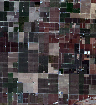
- The images display in the view. All of the images cover the same geographic extent. Here is an example true-color image from November 27, 2020:
The Layer Manager lists all of the files that are in the current view:
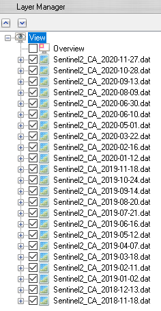
To view an image, enable the check box for the layer to view and uncheck all other layers.
- Click the Data Manager button
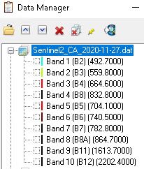
 in the ENVI toolbar. The Data Manager lists all of the bands that comprise each image. The numbers in parentheses are the band wavelengths (in nanometers). You can see that each image has 10 bands, which range from blue to shortwave-infrared (SWIR) wavelengths.
Next, you will explore the data values in an image.
- Click the check box next to Sentinel2_CA_2020-11-27.dat in the Layer Manager, and click on the layer name to make it the active layer.
- Right-click in the middle segment of the Status bar (located at the bottom of the application) and select Raster Data Values.
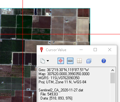
- Move the cursor around the November 27 image, and look at the "Data" values in the Status bar. These are the pixel values in the red, green, and blue bands; for example:
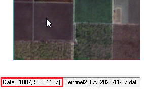
Since this is a Level-1C image, the pixel values represent top-of-atmosphere (TOA) reflectance. They are unsigned integers, scaled by 10,000. For example, a pixel value of 1087 represents a reflectance value of 0.1087, or about 10% reflectance.
- Click the Cursor Value button
 in the ENVI toolbar. The Cursor Value dialog appears, and red crosshairs appear in the view.
- In the Go To field in the ENVI toolbar, enter pixel coordinates 549, 83 and press the Enter key. The crosshairs move to a green field in the upper-right part of the image:
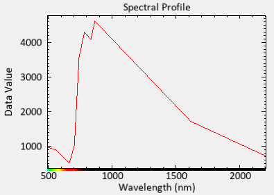
- Right-click on Sentinel2_CA_2020-11-27.dat in the Layer Manager and select Profiles > Spectral. A Spectral Profile window appears, showing a plot of pixel spectral values across all 10 bands in the image. The field where the crosshairs are centered contains healthy, green crops. The spectral profile confirms this because the shape of the plot is typical of healthy vegetation, with an abrupt increase from red to near-infrared reflectance:
- Close the Spectral Profile and Cursor Value dialogs.
While you could use TOA reflectance data to infer crop health, a vegetation index would be better. To do this, the pixel values must be converted to surface reflectance. In the next section, you will build a model to process the data in this manner.
Build a Time Series of Processed Images
The ENVI Modeler provides a quick and simple way to batch-process and construct a time series from multiple images. The model you are about to run will perform the following tasks:
- QUick Atmospheric Correction (QUAC): This task yields surface reflectance data, 0 to 100%. QUAC produces unsigned integer values, so pixels will range from 0 to 10,000. The ENVI Atmospheric Correction Module is required to use this task. If you do not have a license for the ENVI Atmospheric Correction Module, you can substitute another task such as Dark Subtraction.
- Apply Gain and Offset: This task multiplies pixel values by 0.0001 to yield values that range from 0 to 1.0.
- Spectral Indices: A vegetation index can be helpful in assessing the relative health and greenness of crops. The Normalized Difference Vegetation Index (NDVI) is a common broadband index used to assess vegetation health; however, since Sentinel-2 provides three red-edge bands, you should consider using an index that takes advantage of these wavelength regions. Bands that lie along the red edge region are more sensitive to small changes in vegetation foliage content and greenness. They can often indicate early onset of vegetation stress. The Red Edge Normalized Difference Vegetation Index (RENDVI) is an example of an index that can be used for precision agriculture, forest monitoring, and vegetation stress detection. With Sentinel-2, it computes the normalized difference of Bands 5 (704.1 nm) and 6 (740.5):
RENDVI = (B6 - B5) / (B6 + B5)
Pixel values will range from -1 to 1.
- Build Raster Series: This task builds a time series from the spectral index images.
- Extract Rasters From Raster Series: This task extracts the 23 images that comprise the time series and passes them to the next task.
- Build Layer Stack: This task assembles all of the time series images and puts them into one image, where each band represents a vegetation index image from a specific date.
The model will create both a raster series file (.series) and a layer-stacked image (.dat) that you will analyze later.
Explore the Model
- From the ENVI menu bar, select Display > ENVI Modeler. The ENVI Modeler appears.
- Click the Open button in the ENVI Modeler toolbar. The Select Input Model File dialog appears.
- Navigate to the directory where you saved the tutorial data, and select the file Build Time Series.model. Click Open. The model appears in the layout window:
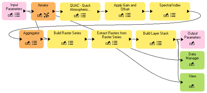
In general, this is how the model works. When you run the model, the pink Input Parameters node will allow you to select the input rasters, along with the locations and filenames for the output raster series file and layer-stacked file. The orange Iterator node will iterately perform QUAC, Apply Gain and Offset, and Spectral Index (in that order) for all of the input files you specify. The orange Aggregator node collects the output from each iteration and stores it in one place. The Build Raster Series task node takes the processed images from the Aggregator node and constructs a time series from them. At the same time, the rasters that comprise the time series will be layer stacked into one image. Both the raster series and the layer-stacked raster are written to disk, added to the Data Manager, and displayed in the ENVI view.
To see the parameters used in each task, click the  buttons in the yellow task nodes. The following parameters were used for this model:
- In the QUAC task node, the Sensor Type is set to Generic / Unknown Sensor. Since Sentinel-2 is not an available option for QUAC, the generic option will suffice. Also, the output is set to Virtual Raster. You do not need to create a file on disk from this task, as the output will be passed directly to the next task.
- In the Apply Gain and Offset task node, the Gain Values field is set to a 10-element array of 0.0001 values. This will multiply the preceding QUAC pixel values by 0.0001 to scale the pixel values from 0 to 1.0 surface reflectance. The Offset Values field is set to a 10-element array of 0 values. Offsets do not need to be applied. The output is set to Virtual Raster.
- In the Spectral Index task node, the Index field is set to Red Edge Normalized Difference Vegetation Index. The output is set to File instead of Virtual Raster. Any task that precedes the Build Raster Series task needs to write its output to a file.
- Nothing was changed in the Build Raster Series, Extract Rasters from Raster Series, and Build Layer Stack nodes. Default values were used.
Run the Model
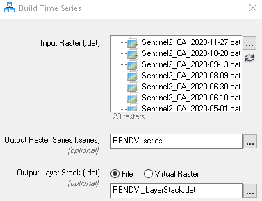
- Click the Run button at the top of the ENVI Modeler. After a few seconds, the Build Time Series dialog appears.
- Click the Browse button
 next to the Input Raster (.dat) field. The Data Selection dialog appears.
- Click the Select All button, then click OK.
- Click the Browse button next to the Output Raster Series (.series) field. The Select Output Raster Series dialog appears.
- Navigate to a directory where you want to save output files. Name the file RENDVI.series, then click Open.
- In the Build Time Series dialog, select the File radio button.
- Click the Browse button next to the Output Layer Stack (.dat) field. The Select Output Layer Stack (.dat) dialog appears.
- In your output directory, name the file RENDVI_LayerStack.dat. Click Open.
- Click OK in the Build Time Series dialog.
The model takes a few minutes to run. When it is finished, the RENDVI raster series and RENDVI layer stack are added to the Data Manager and Layer Manager. They are also displayed in the ENVI view.
- Select File > Exit from the ENVI Modeler menu to close the dialog.
Update Band Names
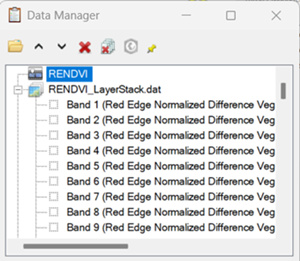
- Open the Data Manager and expand the contents of RENDVI_LayerStack.dat. Each band represents an RENDVI image from a specific data, but the band names are generic and do not indicate dates. This makes it difficult to tell which band corresponds to what date. You will update the band names next.
- In the search window of the ENVI Toolbox (located in the upper-right part of the application), type edit envi and press Enter.
- Double-click the Edit ENVI Header tool. You will use this tool to edit the band names. The Data Selection dialog appears.
- Select the RENDVI_LayerStack.dat file and click OK. The Edit ENVI Header dialog appears.
- Select the Display tab of the dialog.
- In the Band Names field, select the first entry, Band 1.... The band name appears in an Edit field below the Band Names field.
- In the Edit field, enter 2018-11-18 as the new band name, then press the Enter key.
- Do the same with the remaining band names, replacing them as follows:
|
Original band name
|
New band name
|
|
Band 2 |
2018-12-13
|
|
Band 3 |
2019-01-02
|
|
Band 4 |
2019-02-11
|
|
Band 5 |
2019-03-18
|
|
Band 6 |
2019-04-07
|
|
Band 7 |
2019-05-19
|
|
Band 8 |
2019-06-16
|
|
Band 9 |
2019-07-19
|
|
Band 10 |
2019-08-20
|
|
Band 11 |
2019-09-14
|
|
Band 12 |
2019-10-24
|
|
Band 13 |
2019-11-18
|
|
Band 14 |
2020-01-12
|
|
Band 15 |
2020-02-16
|
|
Band 16 |
2020-03-22
|
|
Band 17 |
2020-05-01
|
|
Band 18 |
2020-06-10
|
|
Band 19 |
2020-06-30
|
|
Band 20 |
2020-08-09
|
|
Band 21 |
2020-09-13
|
|
Band 22 |
2020-10-28
|
|
Band 23 |
2020-11-27
|
- Select the Main tab in the dialog.
- In the Description field, replace the default text with Red Edge Normalized Difference Vegetation Index.
- Click the Add button
 . The Add Metadata Items dialog appears.
- Select the Data Ignore Value item, then click OK.
- Set the Data Ignore Value field to -9.9999.
- Click OK in the Edit ENVI Header dialog. The image closes, then reopens and redisplays.
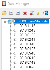
- Check that the band names are correct in the Data Manager.
Now you are ready to begin analyzing the time series.
Analyze the Time Series
The Landsat Time Series Tutorial (available in ENVI Help) describes how to view and animate a time series. Refer to that tutorial for more information on how to use the Series Manager. For this tutorial, you will explore other ways to analyze a time series, rather than simply viewing and animating its images.
View a Time Series Profile
A time series profile is a plot of data values for a given pixel over time. In this case, a time series profile will show RENDVI values for a selected point from November 2018 to November 2020. It can be useful for studying vegetation greenness and health over time.
- Right-click on the [1/23] Spectral_Index_output_raster_2428946747.dat layer in the Layer Manager (the one with a red "1" box), and select Profiles > Series. A Series Profile plot window appears, and red crosshairs appear in the view; for example:
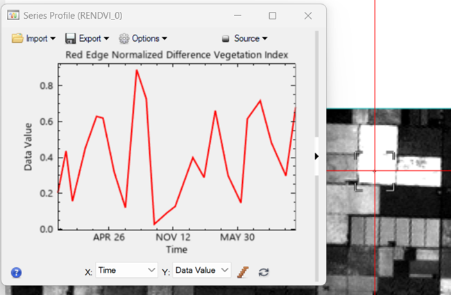
The series profile shows RENDVI values (y-axis) over time (x-axis) for the pixel location indicated by the crosshairs. In the example above, you can see that the crop health for the selected pixel starts out low, then increases in April. It decreases again, then increases in the following spring.
The month and day format is confusing because you cannot tell which year the dates correspond to. In the next step you will change the date format.
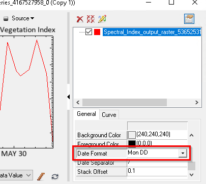
- Click the Show arrow on the right side of the Series Profile. This expands the plot so you can view and edit its properties.
- Under the General tab, scroll down to the Date Format field.
- Click inside of the Date Format field. A drop-down arrow appears.
-
Select YYYY MM DD. The x-axis date format changes.
- Click on different pixels in the image to view time series plots for those locations. Can you find any fields where there appears to be an upward or downward trend in crop health over a two-year period?
Here are some examples. Type the following pixel coordinates into Go To field in the ENVI toolbar, then press the Enter key to jump to these locations:
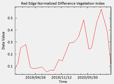
- Location 695, 764 shows an upward trend in crop health:
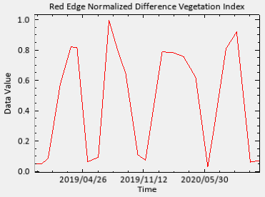
- Location 15, 65 shows an example of a crop with a more frequent growing and harvesting cycle:
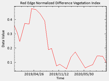
- Location 154, 279 shows an example with a downward trend in crop health:
- When you are finished viewing the plots, close the Series Profile.
In summary, you can use time series profiles to infer trends in crop health and growing cycles, based on a spectral index. A longer time series may reveal more information about drought conditions or other factors that affect crop health.
In addition to viewing the images that comprise a time series and evaluating series profiles, you can use other tools in ENVI to look for trends over time. One such example is performing an unsupervised classification to look for spatial patterns of crop health across a given study area.
Run ISODATA Classification
Unsupervised classification methods such as ISODATA iteratively cluster pixels into different groups according to their statistical information. They do not require any ground truth. Supervised classification, on the other hand, would require a large number of field samples for ground truth. An unsupervised classification only relies on spectral information to group image features based on their statistical information.
ISODATA is an unsupervised method that is widely used in land cover and crop classification, but it is mostly used with spectral bands in imagery. In this exercise, you will use classify the monthly RENDVI bands in the layer-stacked image. While the results do not provide an absolute measure of crop health or crop types, they can reveal some interesting patterns and can indicate fields that share common characteristics.
- In the search window of the ENVI Toolbox, type isodata.
- Double-click the IsoData Classification tool. The ISODATA Classification dialog appears.
- Click the Browse button next to the Input Raster field. The Data Selection dialog appears.
- Select RENDVI_LayerStack.dat and click OK.
- Change the Number of Classes to 12.
- Leave the Change Threshold Percent and Iterations parameters at their default values.
- Click the Browse button next to Output Raster. The Data Selection dialog appears.
- In your output directory, name the classification file RENDVI_Isodata.dat, then click Save.
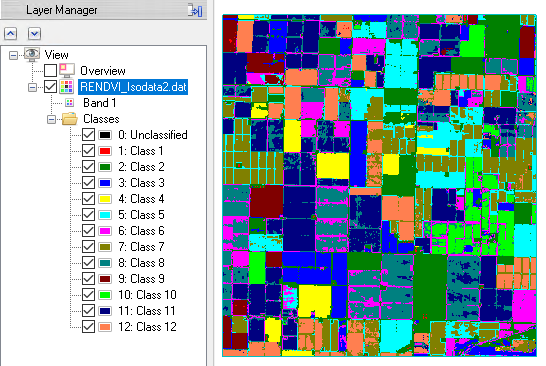
- Click OK in the ISODATA Classification dialog. When processing is complete, the classification image appears in the view. Here is an example. Results may vary:
- This concludes the tutorial. When you are finished, exit ENVI.
See Also
Landsat Time Series Tutorial, Spatiotemporal Analysis, Visual Programming with the ENVI Modeler