This tutorial shows how to create various burn index images from Landsat 8 imagery, using the May 2014 San Diego County wildfires as a case study. You will learn how to perform the following tasks:
- Create binary masks to exclude water pixels
- Calibrate multispectral data to top-of-atmosphere reflectance
- Calibrate thermal data to brightness temperatures
- Create a layer-stacked image that includes the corrected multispectral and thermal bands
- Create burn index images using ENVI's Spectral Index tool
See the following sections:
Files Used in this Tutorial
Tutorial files are available from our ENVI Tutorials web page. Click the Landsat Case Studies link to download the .zip file to your machine, then unzip the files. You will use these files located in the BurnIndices folder the for the tutorial:
|
File |
Description |
|
PostFireOLISubset.dat (and .hdr)
|
Landsat 8 OLI bands (seven total), acquired on May 25, 2014, saved to ENVI raster format.
|
|
PostFireTIRSubset.dat (and .hdr)
|
Landsat 8 TIR thermal bands (two total), acquired on May 25, 2014, saved to ENVI raster format.
|
|
PreFireNBR.dat (and .hdr)
|
Normalized Burn Ratio image from May 9, 2014
|
Data are available from the U.S. Geological Survey.
Case Study: San Diego County Wildfires in 2014
In May of 2014, close to 20 different wildfires erupted in San Diego County, triggered by Santa Ana winds and a heat wave. The first fire started on May 5, and the last remaining fires were extinguished by May 22. By May 18, the fires had burned more than 27,000 acres (42 square miles) of land (Figueroa and Winkley, 2014). Some of the communities affected by the fire included Camp Pendleton, Carlsbad, San Marcos, and Escondido.
Reference: Figueroa, T., and L. Winkley. "Fires in North County closer to being out." San Diego Union Tribune, updated 19 May 2014. http://www.utsandiego.com/news/2014/may/18/Regions-wildfires-closer-to-out-as-weather-shifts/. Accessed June 2014.
Background on Burn Indices
Land resource managers and fire officials use burn severity maps from remote sensing instruments to predict areas of potential fire hazards, to map fire perimeters, and to study areas of vegetation regrowth after fires. Landsat imagery has traditionally been used to create indices that indicate burn severity because of its repeated coverage, ease of access, and spectral wavelengths.
In this tutorial, you will create burn severity images using a variety of different indices.
Burn Area Index
The Burn Area Index (BAI) highlights burned land in the red to near-infrared (NIR) spectrum, by emphasizing the charcoal signal in post-fire images. The index is computed from the spectral distance from each pixel to a reference spectral point, where recently burned areas converge. Brighter pixels indicate burned areas. BAI is computed as follows (Martín, 1998):
Normalized Burn Ratio
This index highlights burned areas in large fire zones greater than 500 acres. The formula is similar to a normalized difference vegetation index (NDVI), except that it uses near-infrared (NIR) and shortwave-infrared (SWIR) wavelengths (Lopez, 1991; Key and Benson, 1995).
The NBR was originally developed for use with Landsat TM and ETM+ bands 4 and 7, but it will work with any multispectral sensor (including Landsat 8) with a NIR band between 0.76-0.9 µm and a SWIR band between 2.08-2.35 µm.
Normalized Burn Ratio - Thermal
This index uses a thermal band to enhance the NBR. It results in a better separability between burned and unburned land (Holden et al., 2005).
NBRT1 was originally developed for use with Landsat TM and ETM+ bands 4, 7, and 6. However, it will work with any multispectral sensor (including Landsat 8) with bands that fall within the following ranges:
- NIR: 0.76 to 0.9 µm
- SWIR: 2.08 to 2.35 µm
- Thermal: 10.4 to 12.5 µm
References:
Holden, Z., et al. "Evaluation of Novel Thermally Enhanced Spectral Indices for Mapping Fire Perimeters and Comparisons with Fire Atlas Data." International Journal of Remote Sensing 26 (2005): 4801-4808.
Key, C. and N. Benson. "Landscape Assessment: Remote sensing of severity, the Normalized Burn Ratio; and ground measure of severity, the Composite Burn Index." In FIREMON: Fire Effects Monitoring and Inventory System, RMRS-GTR, Ogden, UT: USDA Forest Service, Rocky Mountain Research Station (2005).
Lopez Garcia, M.J., and Caselles, V. "Mapping Burns and Natural Reforestation using Thematic Mapper Data. Geocarto International 6 (1991): 31-37.
Martín, M. Cartografía e inventario de incendios forestales en la Península Iberica a partir de imágenes NOAA AVHRR. Doctoral thesis, Universidad de Alcalá, Alcalá de Henares (1998).
Display the Post-Fire Image
Follow these steps to begin:
- From the menu bar, select File > Open. The Open dialog appears.
- Navigate to where you saved the \LandsatCaseStudies\BurnIndices tutorial data and select the PostFireOLISubset.dat file, then click Open.
-
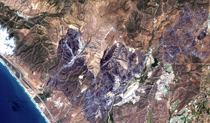
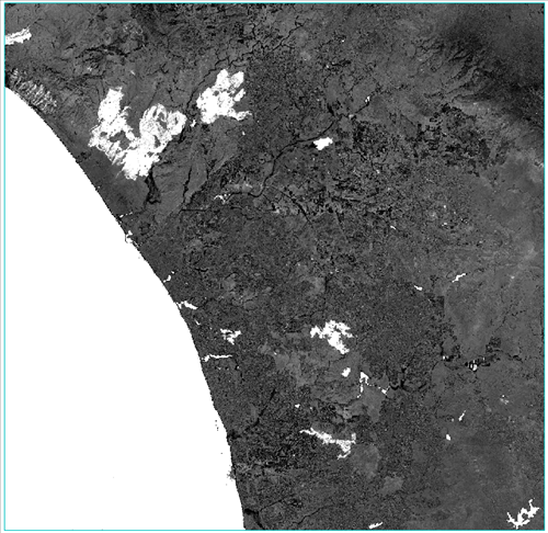
Right-click on the layer name in the Layer Manager and select Zoom to Layer Extent. This multispectral image shows the California coastline from San Clemente in the north to Del Mar in the south. You can see some of the larger burn scars near Camp Pendleton in the upper-left part of the image; they have a distinct gray color. If you cannot clearly see them, choose a different stretch type from the drop-down list in the toolbar:
Tip: This image is a spatial subset of a full Landsat 8 scene. To open full scenes distributed by the U.S. Geological Survey, select the *MTL.txt metadata file. The seven OLI bands are grouped separately from the two TIR thermal bands, Cirrus band, and Quality band. This particular image was created by selecting File > Save As from the menu bar, selecting the OLI band group, defining a spatial subset, and saving the result to ENVI raster format. The thermal bands were similarly saved to a separate file for use with the Calibrate Thermal Bands section of this tutorial.
Preprocessing
Preprocessing steps ensure that the images are properly masked and calibrated before computing burn indices. Not all of the steps below are required in every case study; exceptions are noted below.
Create a Water Mask
Scenes that contain oceans or other large water bodies should be masked to exclude these pixels, as they can interfere with calibration and atmospheric correction. Full Landsat 8 scenes also contain black background pixels that ENVI automatically sets to values of 'NoData'. The sample images you will use in this tutorial have already been spatially subsetted and do not include any background pixels.
An effective way to create a water mask is to create a band-thresholded region of interest (ROI), using the near-infrared (NIR) band. Water has an extremely low reflectance in the NIR region, so those pixels are nearly black. You can isolate those pixels with the ROI Tool.
- In the Layer Manager, right-click on the PostFireOLISubset.dat layer name, and select New Region of Interest. The Region of Interest Tool appears.
- Change the ROI Name to Water.
- Select the Threshold tab.
- Click the Add New Threshold Rule button
 . The Data Selection dialog appears.
- In the Data Selection dialog, select the Near Infrared (NIR) band and click OK. The Choose Threshold dialog appears with a histogram of the NIR band. You will identify the water pixels by selecting the range of low pixel values in the histogram.
- Click and drag the red line on the left edge of the plot toward the right, covering the data values from 0 to approximately 7,618:
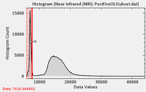
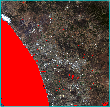
- Enable the Preview check box. The pixels that fall within this range are highlighted in the view in red.
Tip: You can also use ROI thresholds to highlight clouds, using the highest data values in the histogram. However, you will ignore the sporadic cloud cover for this tutorial.
- Click OK in the Choose Threshold dialog. Next, you will mask out the water pixels.
- From the ENVI menu bar, select File > Save As > Save As (ENVI, NITF, TIFF, DTED). The Data Selection Dialog appears.
- Highlight PostFireOLISubset.dat.
- Click the Mask button near the bottom of the dialog. The Mask Selection dialog appears.
- Select Water under the Select mask source(s) area..
- Enable the Inverse mask check box, and click OK.
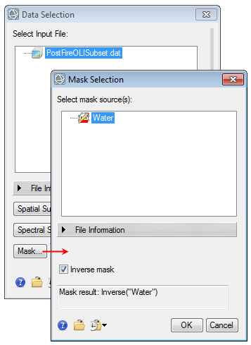
- Click OK in the Data Selection dialog. The Save File As dialog appears.
- Enter 0 for the Data Ignore Value.
- In the Output Filename field, select the directory to save the file to and use PostFireOLISubsetMasked.dat as the filename.
- Enable the Display result check box.
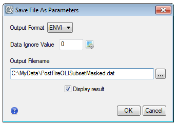
- Click OK.
- After processing is complete, uncheck the PostFireOLISubset.dat layer in the Layer Manager so that only PostFireOLISubsetMasked.dat layer will be visible in the view.
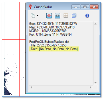
- Click the Cursor Value icon
 in the ENVI toolbar.
- Move the red crosshairs over the white ocean pixels, and verify that the Cursor Value dialog reports NoData values for those pixels:
- Close the Cursor Value dialog.
- Close the Region of Interest Tool.
- Right-click on the View entry in the Layer Manager and select Remove All Layers.
Calibrate OLI Bands to Reflectance
To create spectral index images such as Burn Area Index and Normalized Burn Ratio, the source images should be calibrated to top-of-atmosphere (TOA) reflectance, where pixel values range from 0 to 1.0 or 0 to 100.
Tip: If you wish to create a surface reflectance images, you can use the Dark Subtraction, Flat Field, or IARR tools.
- In the search window of the Toolbox, type calibration. Double-click the Radiometric Calibration tool name that appears.
- Click the Browse button
 next to the Input Raster field. The Data Selection dialog appears.
- Select the file PostFireOLISubsetMasked.dat, and click OK.
- In the Radiometric Calibration dialog, select Top-of-Atmosphere Reflectance from the Calibration Type drop-down list.
- Keep the default selections for all other settings.
- In the Output Raster field, enter the filename PostFireReflectance.dat.
- Click OK.
Calibrate Thermal Bands to Brightness Temperatures
This step is only required for creating a Normalized Burn Ratio - Thermal image, which this tutorial covers. Since Landsat thermal bands are not used for the Burn Area Index or Normalized Burn Ratio Index, so you do not need to calibrate the thermal bands or perform layer stacking for those indices. You do not need to create a water mask for the thermal bands.
Perform these steps to calibrate the thermal bands to brightness temperatures (in Kelvins):
- From the menu bar, select File > Open.
- Navigate to where you saved the \LandsatCaseStudies\BurnIndices tutorial data and select the file PostFireTIRSubset.dat, then click Open. The Thermal Infrared 1 band appears in the display.
- In the search window of the Toolbox, type calibration. Double-click the Radiometric Calibration tool name.
- Click the Browse button next to the Input Raster field. The Data Selection dialog appears.
- Select the file PostFireTIRSubset.dat, and click OK.
- In the Radiometric Calibration dialog, select Brightness Temperature from the Calibration Type drop-down list.
- Keep the default selections for all other settings.
- In the Output Raster field, enter the filename PostFireTIRCalibrated.dat.
- Click OK.
Create a Layer-Stacked Image
These steps will combine the calibrated thermal and OLI bands into one file. You will use the Spectral Indices and Band Math tools later to create a Normalized Burn Ratio - Thermal image. You do not need to build layer stacks to compute Burn Area Index or Normalized Burn Ratio spectral indices.
- In the search window of the Toolbox, type layer stack. Double-click the Build Layer Stack tool name that appears.
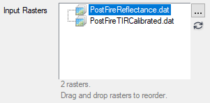
- In the Build Layer Stack dialog, click the Browse button next to the Input Rasters field.
- In the Data Selection dialog, use the Ctrl key on your keyboard to select PostFireTIRCalibrated.dat, and PostFireReflectance.dat . Click OK.
- In the Input Rasters area, PostFireReflectance.dat should be above PostFireTIRCalibrated.dat. Click and drag to move the file order if needed.
- From the Resampling drop-down list, select Cubic Convolution.
- Keep the remaining parameters at their default settings.
- In the Output Raster field, enter the filename PostFireLayerStack.dat.
- Click OK.
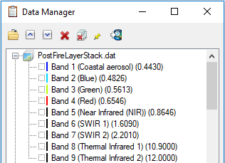
- When processing is complete, click the Data Manager icon
 in the toolbar.
- Verify that the layer stack includes seven OLI bands and two TIR bands.
- Leave the Data Manager open.
Create Burn Index Images
ENVI's Spectral Index tool creates images that represent different indices such as vegetation, burned areas, geologic, and built-up features. You must run this tool each time you create an index image. Follow these steps to compute burn indices:
- In the search window of the toolbox, type spectral indices. Double-click the Spectral Indices tool name. The Data Selection dialog appears.
- Select the file PostFireLayerStack.dat, and click OK.
- In the Index list, select Burn Area Index.
- In the Output Raster field, enter the filename BAI.dat, and click OK.
- Repeat Steps 1-4 for the following indices:
- Normalized Burn Ratio (output filename: PostFireNBR.dat)
- Normalized Burn Ratio Thermal 1 (output filename: NBRT1.dat)
- In the Layer Manager, right-click View and select Remove All Layers.
- From the menu bar, select Views > 2x2 Views. Four empty views appear in the display.
- Drag and drop the BAI.dat Burn Area Index band from the Data Manager to the upper-left view.
- Drag and drop the PostFireNBR.dat Normalized Burn Ratio band from the Data Manager to the upper-right view.
- Drag and drop the NBRT1.dat Normalized Burn Ratio Thermal 1 band from the Data Manager to the lower-left view.
- From the menu bar, select Views > Link Views.
- The Geo Link option already is already selected. Click Link All, then click OK. All three views center over the same geographic location.
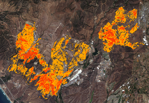
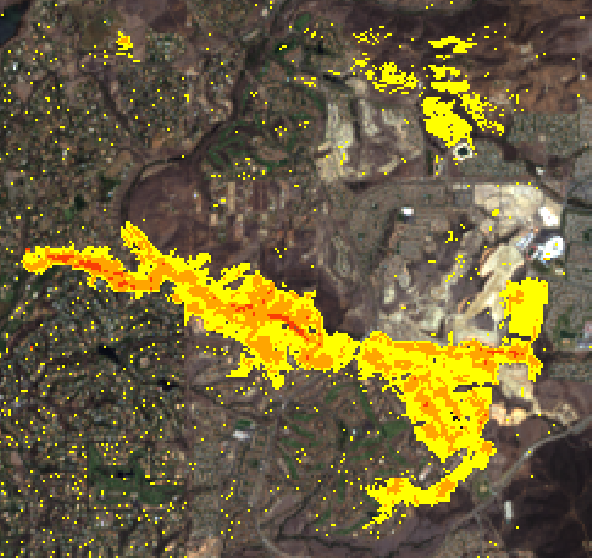
- In the Go To field of the toolbar, type the pixel coordinates 631, 472 and press the Enter key. The views center over the burned region near Camp Pendleton.
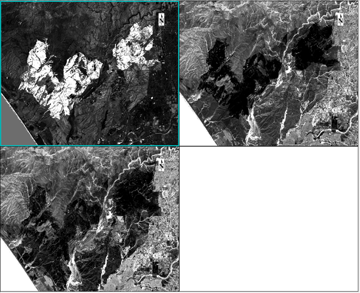
Notice that the brighter pixels in the Burn Area Index image (upper-left view) indicate burned areas, while darker pixels indicate burned areas in the Normalized Burn Ratio images.
- Enter the following pixel coordinates in the Go To field to explore other burned areas:
- 1214, 530 (Fallbrook)
- 1263, 1669 and 873, 1260 (Carlsbad)
- 1246, 1253 (San Marcos)
- 58, 123 (Camp Pendleton)
- Use the navigation, zoom, and stretch tools in the toolbar to further explore the images. How are the Normalized Burn Ratio and its thermal version different from each other? Does one separate burned areas better than the other?
- When you are finished, right-click on each View item in the Layer Manager and select Remove View.
- Close the Layer Manager.
Differenced Normalized Burn Ratio
A differenced normalized burn ratio (dNBR) is another burn-severity product that measures absolute change in the NBR. You can easily create a dNBR image by performing these steps:
- Create an NBR image immediately before the fire.
- Create an NBR image during, or after the fire.
- Subtract the post-fire NBR image from the pre-fire NBR image.
Brighter pixels indicate higher levels of burn severity.
For this tutorial, these steps have been done for you. Normally you would need to perform all of steps in the Preprocessing section on the pre-fire image (just as you did on the post-fire image).
Follow these steps to create a dNBR image:
- From the menu bar, select File > Open.
- Select the file PreFireNBR.dat, and click OK. The pre-fire NBR image is displayed.
- Type band math in the Search window of the Toolbox, and double-click the Band Math tool name.
- In the Enter an expression field, enter float(b2 - b1).
- Click Add to List, then click OK. The Variables to Band Pairings dialog appears.
- Under Variables used in expression, select B1 - [undefined], then in the Available Bands List, select the Normalized Burn Ratio band for PostFireNBR.dat.
- Under Variables used in expression, select B2 - [undefined], then in the Available Bands List, select the Normalized Burn Ratio band under PreFireNBR.dat.
- Enter an output filename of DifferencedNBR.dat, and click OK. The following image appears, with the white pixels indicating burned areas. (The masked ocean pixels are also colored white.)
The U.S. Geological Survey FIREMON program (Key and Benson, 2005) published categories of burn severity, based on pixel values that have been scaled accordingly:
|
dNBR Values |
Burn Severity |
|
< -0.25 |
High post-fire regrowth
|
|
-0.25 to -0.1 |
Low post-fire regrowth
|
|
-0.1 to 0.1 |
Unburned |
|
0.1 to 0.27 |
Low-severity burn
|
|
0.27 to 0.44 |
Moderate- to low- severity burn
|
|
0.44 to 0.66 |
Moderate- to high-severity burn
|
|
> 0.66 |
High-severity burn
|
The tutorial data includes a density color slice file that you can overlay on the dNBR image.
- Right-click on the DifferencedNBR.dat layer in the Layer Manager and select New Raster Color Slice.
- Select the Band Math band name under DifferencedNBR.dat, and click OK. The Edit Raster Color Slice dialog appears.
- Click the Clear Color Slices button
 .
.
- Click the Restore Color Slices from File button
 and select the file DNBRColorSlice.dsr. Click Open. The image is divided into different colors as defined by this color slice.
- Click OK.
-
In the Layer Manager, uncheck the gray box that represents the range of pixel values from -0.1 to 0.1.
- In the Go To field of the toolbar, type the pixel coordinates 631p,472p and press the Enter key.
- In the Zoom To drop-down menu in the toolbar, enter 125 (%). The display centers over the Camp Pendleton burn area.
-
Now uncheck the purple box (-1 to -0.25) and blue box (-0.25 to -0.1). Only the highest levels of burn severity are displayed.
This concludes the Burn Indices tutorial.