Use Topographic Modeling to create shaded relief surfaces from digital elevation data and to extract parameters such as slope, aspect, and their derivatives.
You can also run a script to perform topographic modeling using the TopographicModeling task.
See the following sections:
Background
This section provides an overview of slope, aspect, and other parameters that are used in topographic modeling. For a more detailed background, consult the references at the end of this topic.
For every point in a digital elevation model (DEM), you can compute a number of parameters that represent the change in surface relative to neighboring points. A moving window, or kernel, is used for this purpose. The kernel is used to fit a quadratic surface to the DEM and to derive the appropriate parameters. Varying the size of the kernel allows measurements at various scales. The quadratic surface takes the following form:

Slope
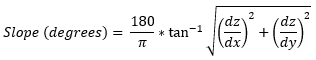
Slope represents the change in elevation (dz) over a given distance (dx). More specifically, it measures the maximum rate of change in elevation between a given point and its surrounding points. ENVI computes slope both in degrees and percentages. Values range from 0 (a horizontal plane) to 90 degrees.
Aspect
Aspect is the compass direction that a slope is facing. Values range from 0 (north) to 360 degrees, increasing in a clockwise direction. ENVI assigns a value of 180 to pixels whose slope is 0.
Shaded Relief
Shaded relief is computed as the cosine of the incidence angle, which is the angle between a vector pointed toward the sun and a vector normal to the surface. Values range from 0 to 1.

Curvature is the rate of the change of slope; thus, it is the first derivative of slope and the second derivative of the local surface. Upward curvature is called convexity, while downward curvature is called concavity. Two forms of convexity—profile and plan—provide vertical and horizontal orthogonal measures of curvature, respectively. Together, they are used to study how water near the surface accelerates and converges. Following published convention, surface convexity values are given a negative sign.
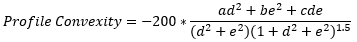
Profile Convexity
Profile Convexity is the vertical component of curvature. It is the curvature of the surface along the steepest downhill direction, where the effects of gravity are maximized. Profile convexity affects the velocity of water flow, and it influences erosion and deposition.
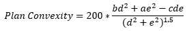
Plan Convexity
Plan Convexity is the horizontal component of curvature. It measures the rate of change of the aspect along a contour, orthogonal to the direction of the steepest slope, where the effects of gravity are minimized.
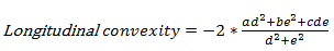
Longitudinal Convexity
Longitudinal Convexity measures the curvature orthogonally in the downslope. It intersects with the plane of the surface normal and the aspect direction. It can determine whether flowing water will accelerate or decelerate over a given point.
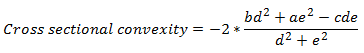
Cross Sectional Convexity
Cross Sectional Convexity measures the curvature orthogonally across the steepest downhill direction. It intersects with the plane of the surface normal and the perpendicular aspect direction. It can determine whether flowing water will converge or diverge over a given point.
In cases where the surface normal is vertical, the convexity measures are undefined and other measures of curvature are used. These are minimum curvature and maximum curvature, shown in the equations below. ENVI assigns convexity values of 0 to pixels whose slope is zero.
Minimum Curvature/Maximum Curvature
Minimum Curvature is the smallest local curvature in any direction. Maximum Curvature is the largest local curvature in any direction. Both measures apply to the entire surface.


RMS
RMS is a root mean square error image that indicates how well the quadratic surface fits the image surface.
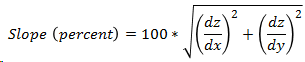
Slope Percent
Slope Percent divides the difference between the elevations of two points (rise) by the distance between them (run), then multiplies the quotient by 100. Values range from 0 to infinity, with a value of 100 indicating a slope of 45 degrees (rise is equal to run).
Run the Topographic Modeling Tool
- From the Toolbox, select Terrain > Topographic Modeling. The Topographic Modeling dialog appears.
- Select a digital elevation image for input. Perform optional spatial subsetting and masking, then click OK.
- Select the Products to create. The choices are as follows (see Background for details on each option):
- Slope
- Aspect
- Shaded Relief
- Profile Convexity
- Plan Convexity
- Longitudinal Convexity
- Cross Sectional Convexity
- Minimum Curvature
- Maximum Curvature
- RMS
- Slope Percent
- Enter the Kernel Size (in pixels) used for processing. The default value is 3 pixels, which represents a 3 x 3 moving window.
- Optional: Enter the Azimuth angle of an illumination source in degrees. The value will only be used for the Shaded Relief product. The default value is 45 degrees.
- Optional: Enter the Elevation angle of an illumination source in degrees. The value will only be used for the Shaded Relief product. The default value is 45 degrees.
- Optional: Enter the X and Y Pixel Size values for the input image in meters. If these values are not set, they will be calculated from the spatial reference of the input image. The default value is 1.0 if the input image does not have a valid spatial reference.
- Enter a filename and location for the Output Raster.
- Enable the Preview check box to preview the settings before processing the data. The preview is calculated only on the area in the view and uses the resolution level at which you are viewing the image. To preview a different area in your image, pan and zoom to the area of interest and re-enable the Preview option. Depending on the algorithm being used by the tool, the preview result might be different from the final result of processing on the full extent, full resolution of the input image in the following scenarios: 1) If you zoomed out of the input raster in the view by 50%, or a percentage less than 50%, ENVI uses a downsampled image at the closest resolution level to calculate the preview, or 2) If the entire image is not visible in the view, ENVI uses the subset in the viewable area of the input image to calculate the preview.
- Enable the Display result check box to display the output in the view when processing is complete. Otherwise, if the check box is disabled, the result can be loaded from the Data Manager.
-
To reuse these task settings in future ENVI sessions, save them to a file. Click the down arrow next to the OK button and select Save Parameter Values, then specify the path and filename to save to. Note that some parameter types, such as rasters, vectors, and ROIs, will not be saved with the file. To apply the saved task settings, click the down arrow  and select Restore Parameter Values, then select the file where you previously stored your settings.
-
To run the process in the background, click the down arrow next to the OK button and select Run Task in the Background. If an ENVI Server has been set up on the network, the Run Task on remote ENVI Server name is also available. The ENVI Server Job Console will show the progress of the job and will provide a link to display the result when processing is complete. See ENVI Servers for more information.
- Click OK.
Example
This example uses a National Elevation Dataset (NED) digital elevation model (DEM), available from the U.S. Geological Survey. The resolution is 1/3-arc seconds with a pixel size of 0.00009259 degrees.
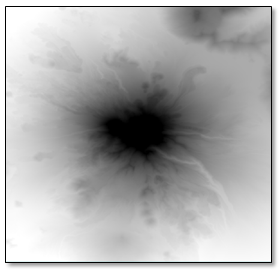
The Topographic Modeling tool was run using default values. The following are the resulting images that were created:
Slope (Degrees)
|
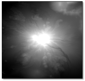
Aspect
|
Shaded Relief
|
Profile Convexity
|
Plan Convexity
|
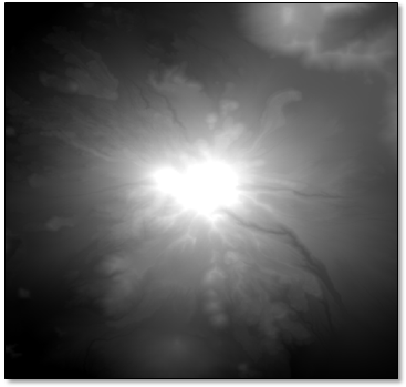
Cross Sectional Convexity
|
Minimum Curvature
|
Maximum Curvature
|
Slope Percent
|
RMS Error
|
References
Evans, I. "General Geomorphometry, Derivatives of Altitude, and Descriptive Statistics." In Spatial Analysis in Geomorphology. Methuen, 1972.
Evans, I. "An Integrated System of Terrain Analysis and Slope Mapping." Zeitschrift für Geomorphologie N.F., Supplement-Band 36 (1980): 274-295.
Goudie, A. Geomorphological Techniques, 2nd Edition. London and New York: Routledge, Taylor & Francis, 1990.
Wood, J. "Scale-Based Characterizations of Digital Elevation Models." In Innovations in GIS 3. Taylor & Francis, 1996.
Wood, J. The Geomorphological Characterization of Digital Elevation Models, Ph.D. Thesis, University of Leicester, Department of Geography, Leicester, UK, 1996.
See Also
Topographic Shading, Extract Topographic Features, Replace Bad Values