Build RPCs
Use the Build RPCs tool to compute rational polynomial coefficient (RPC) information for the following:
- Scanned aerial photographs from a frame camera.
- Digital aerial photographs with a frame central projection (including Vexcel UltraCamD).
- Digital aerial photographs with a line central projection (including Leica ADS40/ADS80 and STARLABO TLS).
- Imagery from any generic pushbroom sensor (including ALOS PRISM and AVINIR, ASTER, Cartosat-1, FORMOSAT-2, GeoEye-1, IKONOS, IRS-C, KOMPSAT-2, MOMS, QuickBird, RapidEye, WorldView-1 and -2, and SPOT) as long as GCPs are available.
RPCs are computed using a digital photogrammetry technique that uses a collinearity equation to construct sensor geometry, where the object point, perspective center, and image point are all on the same space line. The technique involves a series of transformations involving pixel, camera, image-space, and ground coordinate systems.
For single-image orthorectification, the technique includes two preprocessing steps to build the sensor geometry: interior orientation (which transforms the pixel coordinate system to the camera coordinate system), and exterior orientation (which determines the position and angular orientation parameters associated with the image). See Frame and Line Central Projections Background for more information.
Once RPCs are computed, the RPC information is added to the input file header so that you can use the file with DEM Extraction.
You can use the GenerateGCPsFromTiePoints task and use the resulting GCPs in this tool.
Select Input File
- From the Toolbox, select Geometric Correction > Orthorectification > Build RPCs. The Select Input File dialog appears.
- Select an input file such as a scanned aerial photograph, digital aerial imagery, or pushbroom sensor imagery. Click OK. The Build RPCs dialog appears.
- From the Type drop-down list, select one of the following options:
- Frame Camera: Scanned aerial photographs from a frame camera. This is the default value.
- Digital (Frame Central):Digital aerial photographs with a frame central projection. This type of imagery has the same projective geometry as a frame camera but does not include fiducial marks. Examples include Kodak DCS and Vexcel UltraCamD.
- Digital (Line Central): Digital aerial photographs with a line central projection. This type of imagery has one projective center for each sensor image line. Examples include Leica ADS40/ADS80 and STARLABO TLS.
- Pushbroom Sensor: Imagery from any generic pushbroom sensor (including ALOS, ASTER, FORMOSAT-2, IKONOS, IRS-C, KOMPSAT-2, MOMS, QuickBird, RapidEye, and SPOT) as long as GCPs are available. This option may result in better accuracy than the options available through the Map > Orthorectification option in the Toolbox because it uses GCPs (instead of ephemeris data) to compute RPCs. The actual results depend upon the number, the accuracy, and the distribution of GCPs.
The fields and required parameters in the Build RPCs dialog change, depending on the camera Type value you select. The following sections provide more information on each option.
See the following sections for details on parameter settings:
Frame Camera
- From the Type drop-down list in the Build RPCs dialog, select Frame Camera.
- Enter a Focal Length (mm) value for the camera or sensor. This field is required.
- Enter Principal Point x0 (mm) and Principal Point y0 (mm) coordinates, which are usually available from the camera calibration report. The default value is 0 for both fields.
- Click Select Fiducials in Display. The scanned aerial photograph is automatically loaded to a new display group, and the Interior Orientation Fiducials dialog appears.
See the following sections for further steps:
Build Interior Orientation
Interior orientation establishes the relationship between the camera model and the aerial photograph image. It uses tie points between the aerial photograph and the camera fiducial marks (at least four) and the camera focal length.
The options in the Interior Orientation Fiducials dialog are similar to those in the Ground Control Points Selection dialog for image-to-image registration.
- Select a fiducial mark location by centering the mouse cursor (crosshairs) in the Zoom window over it and clicking. The image coordinates appear in the Image X and Image Y fields of the Interior Orientation Fiducials dialog.
- Enter the fiducial location in camera units (mm) in the Fiducial X and Fiducial Y fields. This information should be available in the camera report.
- Click Add Point to add the location to the list of tie points.
- Click Show List to display the Interior Orientation with Fiducials dialog. This dialog is similar to the Image to Image GCP List.
- Continue selecting fiducial mark locations until you have at least four.
- From the Interior Orientation Fiducials dialog menu bar, select Options > Export Fiducials to Build RPCs Widget to compute interior orientation parameters. The Interior Orientation Fiducials dialog closes.
Build Exterior Orientation
- In the Build RPCs dialog, click Select GCPs in Display. The Select GCPs in Display dialog appears.
- Select one of the following options and click OK:
- Restore GCPs from ASCII File: The Enter GCP Filename dialog appears. Select a GCP file that contains projection information (with a .pts extension). Click OK.
- Select Projection for GCPs: The Select GCPs in Display dialog appears. Select a projection type. You can also select Restore GCPs from ASCII File from this dialog. Click OK.
- The Exterior Orientation GCPs dialog appears. This dialog is similar to the Ground Control Points Selection dialog for image-to-map registration.
- Center the crosshairs in the Zoom window over a GCP and click once. The image coordinates appear in the Image X and Image Y fields of the Exterior Orientation GCPs dialog.
- Enter map coordinates for the GCP in the appropriate fields of the Exterior Orientation GCPs dialog.
- In the Elev field, enter an elevation for the selected ground point.
- Click Add Point to add the location to the list of GCPs.
- Click Show List to display the Ground Control Points List . This dialog is similar to the Image to Image GCP List dialog.
- Continue adding GCPs. You should spread the GCPs across the image, including all four corners, for best results. Unlike the GCPs used in “warp” registrations, the accuracy of each GCP used for the exterior orientation is absolutely critical for locating the position of the aerial camera. If the exterior orientation is not accurate, then the orthorectified image will be in error, even if the interior orientation is perfect.
-
From the Exterior Orientation GCPs dialog menu bar, select Options > Export GCPs to Build RPCs Widget to compute exterior orientation parameters. An Exterior Orientation from GCPs Error Report dialog appears, which shows a report of the individual RMS errors for each GCP, and the total RMS error.
The Build RPCs dialog lists six exterior orientation parameters (XS, YS, ZS, Omega, Phi, and Kappa), along with the units of the rotation angles, and the rotation system used.
The rotation matrix associated with XS, YS, and ZS is calculated from three rotation angles: Omega, Phi, and Kappa. While the rotation angles are different among rotation systems, the rotation matrix is the same.
Note: You should only be concerned with the rotation system if you import existing orientation parameters that come from a global positioning system (GPS), inertial navigation system (INS), or inertial measurement unit (IMU); or from block bundle adjustment results using third-party photogrammetry software. If these do not apply to you, then accept the default calculated exterior orientation parameters. Rotation angles are only used to compute the RPCs.
- To edit any of the exterior orientation parameters, click Edit Parameters. The Edit Exterior Orientation Parameters dialog appears. This dialog also allows you to edit the projection information associated with the GCPs.
- From the Rotation System drop-down list in the Edit Exterior Orientation Parameters dialog, select one of the following options.
-
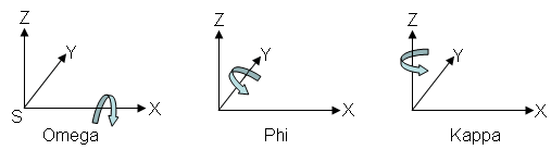
Omega/Phi/Kappa: SX is the primary axis, defined as a fixed axis whose space direction does not change while the direction of the other axes changes as the space is rotated. Omega is a rotation about the SX axis, Phi is a rotation about the SY axis, and Kappa is a rotation about the SZ axis. The following figure shows the positive directions of all the rotation angles. This is the default option since it is widely used in the U.S. and most of the world.
-
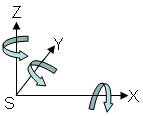
+Phi/Omega/Kappa: SY is the primary axis. Phi is a rotation about the SY axis, Omega is a rotation about the SX axis, and Kappa is a rotation about the SZ axis. The following figure shows the positive directions of all the rotation angles. This convention is commonly used in Germany.
-
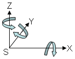
-Phi/Omega/Kappa: This is the same system as +Phi/Omega/Kappa, except the direction of Phi is reversed. This convention is commonly used in China.
- Edit the XS, YS, ZS, Omega, Phi, and Kappa fields in the Edit Exterior Orientation Parameters dialog as needed.
- Click the Units toggle button to toggle between Degrees or Radians. This field represents the units of Omega, Phi, and Kappa.
- Click OK in the Edit Exterior Orientation Parameters dialog.
Compute RPCs
- If you want to further improve the RMS error of the exterior orientation model, click Select GCPs in Display again in the Build RPCs dialog. You can add more GCPs or delete GCPs with large errors.
- When you are finished modifying the GCPs, click Recalculate Exterior Orientation in the Build RPCs dialog.
- Click OK in the Build RPCs dialog. The Scene Elevation in Meters dialog appears.
- The Minimum Elevation and Maximum Elevation fields are initially populated with the range of global elevation values in world_dem (found in the data directory of your ENVI installation path). If you know the elevation range of your scene, you can enter new Minimum Elevation and Maximum Elevation values. These values represent the height above the WGS-84 ellipsoid for the geographic region that the image covers.
-
Click OK. After processing is complete, an ENVI Message dialog appears: “RPCs have been calculated for this file, and the header has been updated.” Click OK.
Once RPCs are computed, the RPC information is added to the input file header so that you can use the file with DEM Extraction.
Digital (Frame Central)
- From the Type drop-down list in the Build RPCs dialog, select Digital (Frame Central).
- Enter a Focal Length (mm) value for the camera or sensor. This field is required.
- Enter Principal Point x0 (mm) and Principal Point y0 (mm) coordinates, which are usually available from the camera calibration report. The default value is 0 for both fields.
- Enter X Pixel Size (mm) and Y Pixel Size (mm) values. These are required fields.
- Click Select GCPs in Display. A Select GCPs in Display dialog appears. See Build Exterior Orientation for the remaining steps.
- If you want to further improve the RMS error of the exterior orientation model, click Select GCPs in Display again. You can add more GCPs or delete GCPs with large errors.
- When you are finished modifying the GCPs, click Recalculate Exterior Orientation in the Build RPCs dialog.
- Click OK. The Scene Elevation in Meters dialog appears.
- The Minimum Elevation and Maximum Elevation fields are initially populated with the range of global elevation values in world_dem (found in the data directory of your ENVI installation path). If you know the elevation range of your scene, you can enter new Minimum Elevation and Maximum Elevation values. These values represent the height above the WGS-84 ellipsoid for the geographic region that the image covers. The minimum and maximum elevations must not be equal for RPCs to build correctly. If they are equal, ENVI will subtract 100 meters from the minimum elevation and will add 100 meters to the maximum elevation.
-
Click OK. After processing is complete, an ENVI Message dialog appears: “RPCs have been calculated for this file, and the header has been updated.” Click OK.
Once RPCs are computed, the RPC information is added to the input file header so that you can use the file with DEM Extraction.
Digital (Line Central)
- From the Type drop-down list in the Build RPCs dialog, select Digital (Line Central).
- Enter a Focal Length (mm) value for the camera or sensor. This field is required.
- Enter Principal Point x0 (mm) and Principal Point y0 (mm) coordinates, which are usually available from the camera calibration report. The default value is 0 for both fields.
- Enter X Pixel Size (mm) and Y Pixel Size (mm) values. These are required fields.
-
Select a Sensor Line Along Axis option. Each sensor line has one projective center.
- X: The sensor line direction is along the image x-axis.
- Y: The sensor line direction is along the image y-axis.
- Set the required Polynomial Orders for XS, YS, ZS, Omega, Phi, and Kappa.
- 0: The parameter is constant for the entire image.
- 1: The parameter has a linear relationship with the y camera coordinates, for example: XS(i) = a0 + a1yi
-
2: The parameter is modeled using a second-order polynomial, for example: XS(i) = a0 + a1yi + a2yi2
The default value is 1 for all six exterior orientation parameters. The higher you set the polynomial order, the more GCPs you must select in the image. Usually, a second-order polynomial is only needed to model a scenario where there is a nonlinear variation of the exterior orientation between sensor lines, which implies an unstable flight path. Experiment with different polynomial orders to select the optimal modeling strategy.
- Click Select GCPs in Display. A Select GCPs in Display dialog appears. See Build Exterior Orientation for the remaining steps.
- If you want to further improve the RMS error of the exterior orientation model, click Select GCPs in Display again. You can add more GCPs or delete GCPs with large errors.
- When you are finished modifying the GCPs, click Recalculate Exterior Orientation in the Build RPCs dialog.
- Click OK. The Scene Elevation in Meters dialog appears.
- The Minimum Elevation and Maximum Elevation fields are initially populated with the range of global elevation values in world_dem (found in the data directory of your ENVI installation path). If you know the elevation range of your scene, you can enter new Minimum Elevation and Maximum Elevation values. These values represent the height above the WGS-84 ellipsoid for the geographic region that the image covers.
-
Click OK. After processing is complete, an ENVI Message dialog appears: “RPCs have been calculated for this file, and the header has been updated.” Click OK.
Once RPCs are computed, the RPC information is added to the input file header so that you can use the file with DEM Extraction.
Pushbroom Sensor
- From the Type drop-down list in the Build RPCs dialog, select Pushbroom Sensor.
- Enter a Focal Length (mm) value for the camera or sensor. This field is required.
- Enter Principal Point x0 (mm) and Principal Point y0 (mm) coordinates.
- Enter X Pixel Size (mm) and Y Pixel Size (mm) values. These are required fields.
- Enter Incidence Angle Along Track and Incidence Angle Across Track values.
- Select a Sensor Line Along Axis option. Each sensor line has one projective center.
- X: The sensor line direction is along the image x-axis.
- Y: The sensor line direction is along the image y-axis.
- Set the required Polynomial Orders for XS, YS, ZS, Omega, Phi, and Kappa.
- 0: The parameter is constant for the entire image.
- 1: The parameter has a linear relationship with the y camera coordinates, for example: XS(i) = a0 + a1yi
- 2: The parameter is modeled using a second-order polynomial, for example: XS(i) = a0 + a1yi + a2yi2
The default value is 1 for all six exterior orientation parameters. The higher you set the polynomial order, the more GCPs you must select in the image. Usually, a second-order polynomial is only needed to model a scenario where there is a nonlinear variation of the exterior orientation between sensor lines, which implies an unstable flight path. Experiment with different polynomial orders to select the optimal modeling strategy.
- Click Select GCPs in Display. A Select GCPs in Display dialog appears. See Build Exterior Orientation for the remaining steps.
- If you want to further improve the RMS error of the exterior orientation model, click Select GCPs in Display again. You can add more GCPs or delete GCPs with large errors.
- When you are finished modifying the GCPs, click Recalculate Exterior Orientation in the Build RPCs dialog.
- Click OK. The Scene Elevation in Meters dialog appears.
- The Minimum Elevation and Maximum Elevation fields are initially populated with the range of global elevation values in world_dem (found in the data directory of your ENVI installation path). If you know the elevation range of your scene, you can enter new Minimum Elevation and Maximum Elevation values. These values represent the height above the WGS-84 ellipsoid for the geographic region that the image covers.
- Click OK. After processing is complete, an ENVI Message dialog appears: “RPCs have been calculated for this file, and the header has been updated.” Click OK.
Once RPCs are computed, the RPC information is added to the input file header so that you can use the file with DEM Extraction.
Parameters for Digital Cameras and Pushbroom Sensors
When building RPCs for digital camera aerial photography and pushbroom sensor imagery, you will need to enter various required parameters such as principal points, focal lengths and pixel sizes, and incidence angles. This section provides guidelines on determining these values.
Principal Point Coordinates
Principal point coordinates are often set to [0.0, 0.0], which assumes that the principal point is the center of the image for a frame central projection, and the center of each scan line for a line central projection. A laboratory calibration report should provide the principal point coordinates.
Focal Length and Pixel Size
Focal length is the orthogonal distance from the perspective center to the image focal plane. Pixel sizes correspond to the CCD cells (detectors of the camera that captured the images). Typically, aerial digital cameras and satellite pushbroom sensors have square pixels, which means that the pixel size is the same in the x and y dimension.
Focal length and pixel sizes are usually available through the data provider or camera calibration report. You can often evaluate the correctness of the input pixel size based on its relationship with flight height, ground resolution, and focal length:
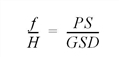
Where:
f is the focal length
H is the aircraft or satellite altitude
PS is the pixel size on the camera lens
GSD is the ground sample distance or ground resolution.
The following table lists focal lengths and pixel sizes for some aerial cameras and satellite pushbroom sensors:
|
Sensor Name |
Focal Length (mm)
|
Image Pixel Size (mm)
|
|
ADS40 |
62.77 |
(0.0065, 0.0065)
|
|
ALOS AVNIR-2 |
800.0 |
(0.0115, 0.0115)
|
|
ALOS PRISM |
1939.0 |
(0.007, 0.007) |
|
ASTER |
329.0 (Bands 1, 2, 3N)
376.3 (Band 3B) |
(0.007, 0.007)
Bands 1, 2, 3N, 3B
|
|
Cartosat-1 |
1945.0 |
(0.007, 0.007) |
|
Deimos-1 |
155.9 |
(0.005, 0.005) |
|
EROS-A1 |
3500.0 |
(0.013, 0.013) |
|
FORMOSAT-2 |
2896.0 |
(0.0065, 0.0065) Pan
|
|
GeoEye-1 |
13300.0 |
(0.008, 0.008) Pan
(0.032, 0.032) Multispectral
|
|
Göktürk-2 |
985.0 |
|
|
IKONOS-2 |
10000.0 |
(0.012, 0.012) Pan
|
|
IRS-1C |
982.0 |
(0.007, 0.007) Pan
|
|
IRS-1D |
974.8 |
(0.007, 0.007) Pan
|
|
KOMPSAT-2 |
9000.0 Pan
2250.0 Multispectral
|
(0.013, 0.013) |
|
KOMPSAT-3 |
8562.0 |
(0.00875, 0.00875) Pan
(0.0175, 0.0175) Multispectral
|
|
Kodak DCS420 |
28.0 |
(0.009, 0.009) |
|
Landsat 8 OLI |
886.0 |
(0.018, 0.018) Pan
(0.036, 0.036), Multispectral
|
|
MOMS-02 |
660.0 |
(0.01, 0.01) |
|
Pleiades-HR |
12905.0 |
(0.013, 0.013) Pan
(0.052, 0.052) Multispectral
|
|
Proba-V (VGT-P) |
109.6 |
(0.013, 0.013) VNIR
|
|
QuickBird |
8836.2 |
(0.013745, 0.013745)
|
|
RapidEye |
637.0 |
(0.0065, 0.0065)
|
|
ResourceSat AWiFS
|
139.5 |
(0.010, 0.007) |
|
ResourceSat LISS-IV
|
982.0 |
(0.007, 0.007) |
|
ResourceSat LISS-III
|
347.5 |
(0.010, 0.007) VNIR
(0.013, 0.013) SWIR
|
|
SkySat-1 |
3600.0 |
(0.0065, 0.0065)
|
|
SPOT-1 through -4
|
1082.0 |
(0.013, 0.013) Pan
|
|
SPOT-5 HRS |
580.0 |
(0.0065, 0.0065) Pan
|
|
SPOT-6 and -7 |
3760.0 |
(0.008, 0.008) Pan
(0.033, 0.033) Multispectral
|
|
SSOT |
5131.0 |
|
|
STARLABO TLS |
60.0 |
(0.007, 0.007) |
|
UK-DMC-2 |
155.9 |
(0.005, 0.005) |
|
Vexcel UltraCamD
|
101.4 |
(0.009, 0.009) Pan
|
|
VNRedSat-1 |
5131.0 |
(0.012, 0.012) Pan
(0.048, 0.048) Multispectral
|
|
WorldView-2 |
13311.0 |
(0.008, 0.008) |
|
Z/I Imaging DMC |
120.0 |
(0.012, 0.012) |
|
ZY-1-02C |
1010.0 |
(0.0065, 0.0065)
|
Along Track and Across Track Incidence Angles
These parameters only apply to pushbroom sensors, and they are different for each sensor. Data from some pushbroom sensors have fixed incidence angles across all images, while other data have different incidence angles for each image. These angles are only used to set the initial values for the exterior orientation parameters and do not have to be exact.
The along track incidence angle is the angle (in degrees) between the vertical position of the satellite and its forward or backward viewing direction. If viewed from the ground point corresponding to the scene center, the along track incidence angle has a positive value if the viewing direction is northward.
The across track incidence angle is the angle (in degrees) between the vertical position of the satellite and its side-viewing direction when the sensor is scanning along the side. If viewed from the ground point corresponding to the scene center, the across track incidence angle has a positive value if the viewing direction is eastward.
Following are some guidelines for determining the incidence angles for different pushbroom sensors.
ASTER
You can set both angles to 0.0 degrees. However, for Band 3B, you should set the along track incidence angle to -27.6 degrees (descending orbit) or 27 degrees (ascending orbit), and the across track incidence angle to 0.0 degrees.
IKONOS
The *_metadata.txt file associated with an IKONOS dataset lists Nominal Collection Elevation Angle and Nominal GSD (Cross Scan and Along Scan) for each source image. Use these values to compute the approximate along track and across track incidence angles with the following equations:
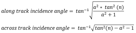
Where:
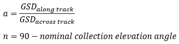
You should set the signs of the incidence angles according to the actual pointing direction, which you can determine from the Nominal Collection Azimuth value in the *_metadata.txt file.
IRS-1C/1D
Set the along track incidence angle to 0.0 degrees. Set the across track incidence angle according to the Input view angle (Deg) value in the leader file.
KOMPSAT-2
Set the approximate incidence angles using the AUX_IMAGE_SATELLITE_INCIDENCE_DEG metadata field in the associated ephemeris data file (.eph).
QuickBird
Set the approximate incidence angles (and signs) using the inTrackViewAngle and crossTrackViewAngle values in the associated *.IMD file.
RapidEye
Set the across track incidence angle to the spaceCraftViewAngle value in the associated *_metadata.xml file. Set the along track incidence angle to 0.0 degrees.
SPOT
Incidence angles are available in the leader file (CAP format) or XML metadata file (DIMAP format).
For SPOT-1 through SPOT-4 data, you can set the along track incidence angle to 0 because this type of viewing is not allowed. For SPOT-5 data, the XML metadata lists the along track incidence angle in the <INCIDENCE_ANGLE> tag. Use the <VIEW_ANGLE> tag to set the across track incidence angle.
For CAP-format data, the incidence angle is in the byte offset 453-468 within the header record. You can use a simple text editor to view the header record. The format for the incidence angle is <X>AA.A, for example, L12.7 or R18.1. If the prefix is L, set the angle to a negative value. If the prefix is R, set the angle to a positive value.
WorldView-1 and WorldView-2
Set the approximate incidence angles (and signs) using the mean InTrackViewAngle and meanCrossTrackViewAngle values in the associated *.IMD file.