This tutorial demonstrates how to read, georeference, and display Sentinel-3 Level-2 Ocean and Land Colour Instrument (OLCI) imagery in ENVI. You will view and reproject marine products such as chlorophyll concentration and water transparency data. You will learn how to apply color tables and how to save a screen capture of the displayed layers to a TIFF file.
See the following sections:
Files Used in This Tutorial
Tutorial files are available from our ENVI Tutorials web page. Click the Sentinel link to download the .zip file to your machine, then unzip the files. The files you will use in this tutorial are located in the S3A_Marine_GulfOman folder of the download.
The dataset used in this tutorial is a Sentinel-3A OLCI Level-2 marine product (OL_2_WFR) with a resolution of 300 meters. It covers a section of the Gulf of Oman and the northern Arabian Sea on 23 December 2017:
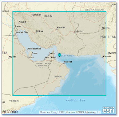
Acknowledgement: Copernicus Sentinel data 2017. Data files are available from the European Organisation for Meteorological Satellites (EUMETSAT), Copernicus Online Data Access site at https://coda.eumetsat.int/#/home.
Sentinel-3 images and metadata are stored in NetCDF-4 format. By opening the xfdumanifest.xml file (see Open a Sentinel-3 File), ENVI automatically reads the standard datasets such as reflectance, algal pigment concentration, etc., and converts them to a raster format that can be displayed in ENVI. The Sentinel-3 package also includes ancillary data that accompanies the imagery.
Background
The Sentinel-3 mission is jointly operated by the European Space Agency (ESA) and EUMETSAT. Its main objective is to measure sea surface topography, sea and land surface temperature, and ocean and land surface color. Sentinel-3 builds on the legacy of ERS-1, ERS-2, and ENVISAT missions to provide ocean forecasting and climate and environmental monitoring.
The OLCI instrument is a pushbroom imaging spectrometer that measures water-leaving reflectance in 21 spectral bands. Its purpose is to measure the distribution of up-welling radiance just above the sea surface. From this, biophysical parameters can be derived for ocean and land surfaces. The most notable is ocean color, which describes the elements and phytoplankton biomass concentration (Chl-a) in water that contribute to its varying color. Coloration can also be impacted by suspended sediment and organic matter, particularly in coastal and shallow waters. Applications of ocean color monitoring include estimating net primary production, studying algal blooms and water quality, and understanding ocean mesoscale and sedimentary processes (ESA, 2013).
The processing steps that you will perform in this tutorial apply not only to ocean color data but to all supported Sentinel-3 data. ENVI supports the following Sentinel-3 products (from ESA, 2013):
Ocean and Land Colour Instrument (OLCI)
|
Label |
Description |
|
OL_1_EFR |
Level-1 top-of-atmosphere (TOA) radiances for each view and each OLCI channel, 300 m resolution.
|
|
OL_1_ERR |
Level-1 TOA radiances for each view and each OLCI channel, 1.2 km resolution.
|
|
OL_2_LFR |
Level-2 land products at 300 m resolution. Land products include Global Vegetation Index (GVI), Terrestrial Chlorophyll Index (TCI), integrated water vapor (IWV) columns, and rectified reflectance for the 681 nm and 865 nm channels.
|
|
OL_2_LRR |
Level-2 land products at 1.2 km resolution.
|
|
OL_2_WFR |
Level-2 marine products at 300 m resolution. Marine products include reflectances in most channels, total backscattering coefficients, total absorption coefficients, algal pigment (chlorophyll) concentration from two different algorithms, total suspended matter concentration, diffuse attenuation coefficients (DACs), colored detrital/dissolved material (CDM), photosynthetically active radiation (PAR), aerosol Angström exponents, and IWV columns.
|
|
OL_2_WRR |
Level-2 marine products at 1.2 km resolution.
|
Sea and Land Surface Temperature Radiometer (SLSTR)
|
Label |
Description |
|
SL_1_RBT |
Level-1 TOA radiances (0.5 km resolution) and brightness temperatures (1 km resolution).
|
|
SL_2_WCT |
Level-2 sea surface temperatures (SSTs); single and dual view, 2 and 3 channels; 1 km resolution.
|
|
SL_2_WST |
Level-2P brightness temperatures, SSTs, sea ice fraction, and wind speed, 1 km resolution. SSTs are based on the Group for High Resolution Sea Surface Temperature (GHRSST) Level-2P specification.
|
|
SL_2_LST |
Level-2 land surface temperatures and associated parameters, 1 km resolution.
|
|
SL_2_AOD |
Level-2 aerosol optical depth, 1 km resolution.
|
In the next section, you will open and explore an OLCI (OL_2_WFR) dataset.
Open a Sentinel-3 File
- Start ENVI.
- From the ENVI menu bar, select File > Open.
-
Navigate to the location where you saved the tutorial data. Go to the Sentinel\S3A_Marine_GulfOman directory. Select the file xfdumanifest.xml and click Open. ENVI initially displays a color image of three reflectance bands.
- Click the Data Manager button
 in the ENVI Toolbar. The Data Manager lists all of the datasets that are currently open. They include the following, from ESA (2013):
|
Dataset |
Description
|
|
Bands 1-21
|
Water-leaving, surface directional reflectance values for all bands except those dedicated to measuring atmospheric gas (i.e., bands Oa13, Oa14, Oa15, Oa19, and Oa20). Reflectance is based on the Baseline Atmospheric Correction (BAC) algorithm, which accounts for atmospheric effects and sun-specular reflection.
|
|
Algal pigment concentration (Neural Net)
|
Chl-a concentration computed using the Inverse Radiative Transfer Model-Neural Network (IRTM-NN) algorithm, described in the Sentinel-3 OLCI Technical Guide (see References), measured in mg / m3.
|
|
Algal pigment concentration
|
Chl-a concentration computed using the OC4Me Maximum Band Ratio (MBR) algorithm developed by Morel et al (2007), measured in mg / m3.
|
|
CDM absorption coefficient (Neural Net)
|
The absorption of colored detrital and dissolved material at 443 nm, measured in m-1.
|
|
Integrated Water Vapour
|
The total amount of water vapor integrated over an atmospheric column, measured in kg / m2 over water only.
|
|
Photosynthetically active radiation
|
Quantum energy flux from the sun in the spectral range 400-700 nm, measured in μEinstein/m2 * 1/s.
|
|
Diffuse attenuation coefficient
|
Downwelling irradiance at 490 nm, measured in m-1. This indicates how much blue/green wavelengths penetrate the water column; thus, it is a measure of turbidity. The algorithm is from Morel (2007).
|
|
Total suspended matter concentration (Neural Net)
|
Concentration of suspended matter in the water, measured in g/m3.
|
|
Aerosol Angström exponent
|
Spectral dependency of the aerosol optical depth between 779 and 865 nm.
|
|
Aerosol optical thickness
|
Aerosol load expressed in the optical depth at 865 nm.
|
The default reflectance image that is currently displayed is not what you will use in this tutorial. You will explore more meaningful datasets next.
- Right-click the S3A_Marine_GulfOman layer in the Layer Manager and select Remove.
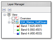
- In the Data Manager, select the Diffuse attenuation coefficient band and click Load Grayscale.
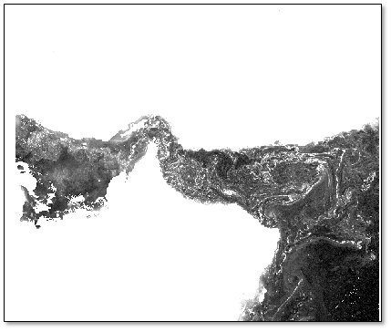
- When the image displays, press the F12 key on your keyboard to view the full extent of the image. It will look similar to the following figure:
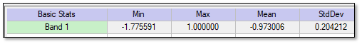
- Right-click on the image layer in the Layer Manager and select Quick Stats. The Statistics View dialog appears.
- In the Basic Stats section, note the minimum and maximum data values in the image. Diffuse attenuation coefficient (DAC) values are measured in m-1.
This image has no spatial context, so you cannot tell where it is located. When you move the cursor inside of the Image window, the center segment of the Status bar (at the bottom of the ENVI application) lists the current projection as "*GLT* Geographic Lat/Lon, WGS-84." This indicates that the geographic coordinates for the image—displayed in the left segment of the Status bar—are derived from a Geographic Lookup Table (GLT) instead of a true map projection. The GLT coordinates are only estimates of geographic locations.
In the next section, you will reproject the DAC and another OLCI dataset to a standard map projection.
Reproject Datasets to a Geographic WGS-84 Projection
ENVI has two tools that reproject GLT datasets to standard map projections. The simplest tool to use with Sentinel-3 data is Reproject GLT with Bowtie Correction. This tool reprojects one band at a time, not the entire dataset.
Note: Bowtie correction is only necessary with MODIS data and will not be applied here.
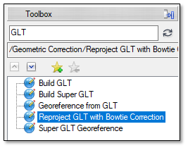
- In the search window of the ENVI Toolbox, type GLT.
- Double-click the Reproject GLT with Bowtie Correction tool name that appears. The Reproject GLT dialog appears.
- Click the Browse button
 next to the Input Raster field. The Data Selection dialog appears.
- Select the Diffuse attenuation coefficient: S3A_Marine_GulfOman raster and click OK. Keep the default selection of Geographic Lat/Lon for Projection Type. The image is in a mid-latitude location, so this projection will be suitable.
- In the Resampling Method, keep the default selection of Distance Weighted. The reprojection will be based on a distance-weighted average of the surrounding valid pixel values. This option results in fewer visible interpolation artifacts, compared to the Nearest Neighbor method.
- Click the Browse button next to Output Raster. Select an output directory for the reprojected image, and name the file DACReprojected.dat.
- Enable the Display result check box.
- Click OK to begin processing. When processing is complete, the reprojected image appears in the view.
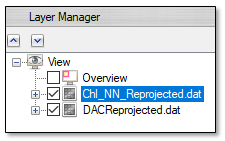
- Repeat Steps 2-8 with the Algal pigment concentration (Neural Net) band. Name the output file Chl_NN_Reprojected.dat.
- When processing is complete, right-click the original Diffuse attenuation coefficient layer in the Layer Manager, and select Remove. Only the two reprojected images remain.
Add Coastlines and Country Boundaries
Next you will overlay coastline and country vectors so that the geographic location of the imagery is more readily apparent.
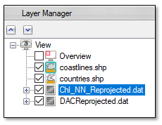
- From the ENVI menu bar, select File > Open World Data > Countries. A vector layer of country boundaries is displayed over the chlorophyll image (Chl_NN_Reprojected.dat).
- From the ENVI menu bar, select File > Open World Data > Coastlines. A vector layer of coastlines is displayed, with the same color as the country boundaries. You will change its color next.
- Double-click the coastlines.shp layer in the Layer Manager. The Vector Properties dialog appears.
- On the right side of the dialog, click inside the Line Color field. When the drop-down arrow appears, click it and select a black color from the color table.
- Click OK.
- Double-click the countries.shp layer in the Layer Manager. The Vector Properties dialog appears.
- Click inside of the Fill Interior field. When the drop-down arrow appears, click it and set the value to True.
- Click inside of the Fill Color field. When the drop-down arrow appears, click it and select a light gray color from the color table.
- Click the Apply button. The countries are filled with a light gray color. If you do not like this color, you can change it as desired.
- Click OK to dismiss the Vector Properties dialog.
The following image shows an example of the grayscale chlorophyll image displayed with country boundaries and coastlines:
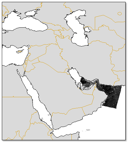
You can toggle between the chlorophyll image (Chl_NN_Reprojected.dat) and the DAC image (DACReprojected.dat) by checking and unchecking their respective boxes in the Layer Manager. Both images are dark, which makes interpretation difficult. In the next section, you will experiment with display enhancements and add color tables so that the images are easier to analyze.
Enhance the Images
- Click the Chl_NN_Reprojected.dat layer in the Layer Manager to make it the active layer.
- Click the Stretch Type drop-down list in the ENVI toolbar and select Square Root.
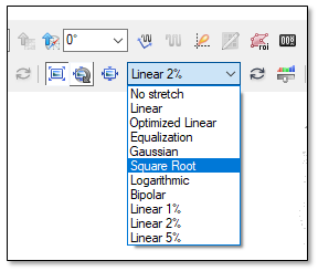
A square root stretch is applied to the chlorophyll image, which brightens it and enhances the circulatory patterns in the water.
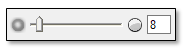
- In the ENVI toolbar, reduce the Sharpness value to 8. This reduces the speckling and noise in the image.
- Right-click on the Chl_NN_Reprojected.dat layer in the Layer Manager and select Change Color Table > More. The Change Color Table dialog appears.
- From the drop-down menu, select the Eos A color table.
- Click OK to dismiss the Change Color Table dialog.
- Click the Cursor Value button
 in the ENVI toolbar.
- Click inside of the chlorophyll image. Red crosshairs are centered over the selected pixel, and the Cursor Value dialog shows the corresponding pixel value in the "Data" line. Pixels with the highest algal pigment concentration (Chl-a) are colored red, while the lowest values are colored blue and black. In the following figure, the selected pixel has a concentration value of -0.71. White areas contain transparent pixels, which have values of "NoData." These correspond to clouds, plus water that is outside of the scene boundary.
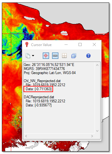
The Cursor Value tool also shows the pixel value for the underlying DAC image. In this example, the value is -0.94. The Cursor Value tool provides a convenient way to view data values of multiple co-registered images at once.
- Dismiss the Cursor Value dialog.
The currently selected color table shows too much red and not enough of the intermediate colors (yellow and green) that represent the majority of the data values. You can try changing the stretch type or color table, but one effective method is to stretch the image histogram.
Stretch the Image Histogram
- Click the Chl_NN_Reprojected.dat layer in the Layer Manager to make it the active layer.
- Click the Histogram Stretch button
 in the ENVI toolbar. The Histogram Stretch dialog appears.
- Drag the right vertical slider all the way to the right so that the stretch includes all of the highest pixel values:
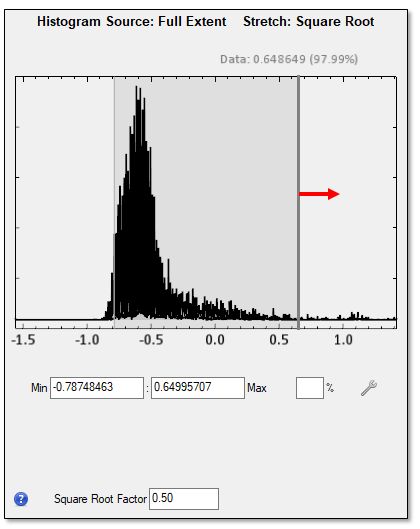
- Make slight adjustments to the left vertical slider (or experiment with lower Min values) so that the stretch includes more green and less blue pixels.
- Set the Square Root Factor value to 0.8.
- Click OK in the Histogram Stretch dialog.
- Zoom into the chlorophyll image to explore the various patterns and colors of the algal pigment concentration.
Add a Color Bar
You can add a color bar to the display by following these steps:
- Click the Annotations drop-down list in the ENVI toolbar and select Color Bar.
- Click inside of the display. The Select Layer dialog appears.
- Select Chl_NN_Reprojected.dat and click OK.
- Resize the color bar and drag it to any location you want.
- Annotation properties are displayed beneath the Toolbox in the lower-right corner of the ENVI application. Click in the Scale on Zoom property field and change the value to False.
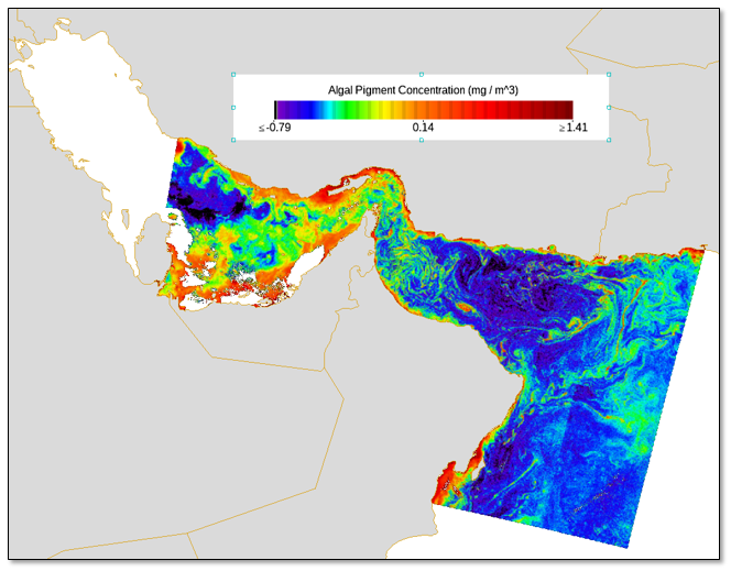
- Change the Title to Algal Pigment Concentration (mg / m^3).
- Change the Font Name to Arimo Regular.
- Increase the Font Size to 12.
To further move or resize the color bar, you must first select the Color Bar item in the Layer Manager. The following figure shows an example of the chlorophyll image at its full extent, along with a color bar annotation:
Tip: To save the current view with all of its image layers and annotations, you can select File > ENVI Session > Save from the ENVI menu bar. Save the view to a .json file on disk. Then you can restore it later and resume your work.
Save a Screen Capture to TIFF Format
You can save a screen capture (called a chip) of the display to an image file on disk by following these steps:
- From the ENVI menu bar, select File > Chip View To > File. The Chip to File Parameters dialog appears.
- From the Output Format drop-down list, select TIFF.
- Select an output filename and location for the TIFF file.
- Enable the Display result check box.
- Click OK.
The screen capture retains the color table, annotations, and display enhancements that you added. It also contains all of the layers present in the Layer Manager. The output TIFF file is an 8-bit, three-band image at screen resolution.
Additional Options
Now that you have learned how to reproject, display, and enhance the DAC and chlorophyll datasets, you can experiment with other datasets. These include total suspended matter concentration, integrated water vapor, and algal pigment (chlorophyll) concentration from the OC4Me algorithm. Here are some additional options to explore:
- Apply different color tables to different datasets.
- Display multiple datasets in separate views, then geographically link them.
- Add grid lines, text annotations, and other map elements to the display. These are available from the Annotations drop-down list.
- Use the File > Chip View To > PowerPoint menu option to send a screen capture of the display to PowerPoint.
References:
European Space Agency. "Sentinel-3 OLCI Technical Guide." https://sentinel.esa.int/web/sentinel/technical-guides/sentinel-3-olci. Accessed March 2018.
European Space Agency. "Sentinel-3 User Handbook." ESA Standard Document, 02 September 2013. https://sentinel.esa.int/documents/247904/685236/Sentinel-3_User_Handbook. Accessed March 2018.
Morel, A., B. Gentili, H. Claustre, M. Babin, A. Bricaud, J. Ras, et al. "Optical Properties of the 'Clearest' Natural Waters." Limnology and Oceanography 52 (2007): 217-229.
List of Acryonms
|
Acronym |
Definition |
|
BAC |
Baseline Atmospheric Correction
|
|
CDM |
Colored Detrital/dissolved Material
|
|
DAC |
Diffuse Attenuation Coefficients
|
|
ESA |
European Space Agency
|
|
EUMETSAT |
European Organisation for Meteorological Satellites
|
|
GHRSST |
Group for High Resolution Sea Surface Temperature
|
|
IRTM-NN |
Inverse Radiative Transfer Model-Neural Network
|
|
IWV |
Integrated Water Vapor
|
|
MBR |
Maximum Band Ratio
|
|
GVI |
Global Vegetation Index
|
|
OLCI |
Ocean and Land Colour Instrument
|
|
PAR |
Photosynthetically Active Radiation
|
|
SST |
Sea Surface Temperature
|
|
SLSTR |
Sea and Land Surface Temperature Radiometer
|
|
TCI |
Terrestrial Chlorophyll Index
|
|
TOA |
Top of Atmosphere
|