In this tutorial, you will use Feature Extraction to extract asphalt surfaces from a multispectral GeoEye-1 scene of a residential area in Hobart, Tasmania. Feature Extraction provides a quick, automated method for identifying roads and parking lots, saving an urban planner or GIS technician from digitizing them by hand. You will learn how various attributes can help you build meaningful rules in classification, and you will export your classification results to a shapefile. If you need more information about a particular step, click the blue Help button to access ENVI Help.
Files Used in This Tutorial
Tutorial files are available from our ENVI Tutorials web page. Click the Feature Extraction link to download the .zip file to your machine, then unzip the files. You will use the file named Hobart_GeoEye_pansharp.dat for this tutorial.
This is a pan-sharpened GeoEye-1 image (0.5-meter spatial resolution) of the Dowsing Point suburb of Hobart, Tasmania, acquired on 05 February 2009. GeoEye-1 images are courtesy of DigitalGlobe.
Background
Feature Extraction uses an object-based approach to classify imagery, where an object (also called a segment) is a group of pixels with similar spectral, spatial, and/or texture attributes. Traditional classification methods are pixel-based, meaning that spectral information in each pixel is used to classify imagery. With high-resolution panchromatic or multispectral imagery, an object-based method offers more flexibility in feature extraction types.
The workflow involves dividing an image into many segments, computing various attributes for the segments, then building rules to classify features of interest. Each rule contains one or more attributes such as area, length, or texture, which you constrain to a specific range of values. For example, we know that roads are elongated, some buildings approximate a rectangular shape, and trees are highly textured compared to grass.
Start the Workflow
- From the menu bar, select File > Open. The Open dialog appears.
- Navigate to feature_extraction, and select the file Hobart_GeoEye_pansharp.dat. Click Open. The image is displayed at full resolution.
- From the Optimized Linear drop-down list in the toolbar, select Linear 5%. This type of stretch brightens the image, making it easier to see individual features.
- From the Toolbox, select Feature Extraction > Rule Based Feature Extraction Workflow. The Data Selection panel appears.
- The filename is already listed in the Raster File field. Click Next. The Object Creation panel appears.
Segment the Image
Segmentation is the process of dividing an image into segments that have similar spectral, spatial, and/or texture characteristics. The segments in the image ideally correspond to real-world features. Effective segmentation ensures accurate classification.
- Enable the Preview option. A Preview Window with segments outlined in green appears over the center of the view (you may need to move the Object Creation panel to see it). The following image (zoomed to 200%) shows an example of a Preview Window centered over some asphalt roads:
The initial segmentation shown in the Preview Window sharply delineates the edges of the roads, but there are too many small segments comprising each road. Use a combination of segmentation and merging to delineate the road boundaries with as few segments as possible. A general rule is to decrease the Scale Level (thus creating more segments) while increasing the Merge Level to merge adjacent segments. It is better to have more segments to delineate your features of interest, but realize that too many segments will result in slower processing.
- Experiment with the different Algorithm options under Segment Settings and Merge Settings, and change the Level for each. The Preview Window automatically updates to show how your changes affect the segmentation.
You can achieve reasonable results with the following settings:
- Segment Algorithm: Edge
- Scale Level: 40
- Click the Select Segment Bands button
 , and select only Band 4. Performing segmentation only on the near-infrared band produces sharper segments on asphalt roads.
- Merge Algorithm: Full Lambda Schedule
- Merge Level: 80
- Texture Kernel Size: 3
The following image shows the resulting segmentation over a road intersection using these settings:
- When you are satisfied with the segmentation, click Next. ENVI creates and displays a segmentation image (also called the Region Means image) in the Layer Manager. Each segment is assigned the mean spectral values of all the pixels that belong to that segment. The Rule-based Classification panel appears.
Build Rules
In this step, you will build several rules to define an Asphalt class. For each segment, ENVI computes various spatial, spectral, and texture attributes. See Spatial, Spectral, and Textural Attributes for definitions of all available attributes.
To decide which attributes to use for identifying asphalt surfaces, consider some characteristics of asphalt in a remote sensing image. Here are some ideas:
- Asphalt roads appear very dark in a near-infrared image, so low spectral mean values in Band 4 should highlight the roads.
- Roads are elongated.
- Roads and parking lots have a uniform texture.
- Smaller features such as rooftops and shadows can also have low spectral values, so you can use an Area attribute to filter out these small segments.
The typical workflow for building rules is to begin with one attribute, test its confidence in extracting your feature of interest, then use more conditions and attributes to filter out all other features from the scene so that you are left only with your feature of interest.
When you combine multiple attributes for a given rule, all of the conditions must apply for the rule to be satisfied.
The Band 4 spectral mean is a good attribute to start with, since most of the roads are very dark in this band.
Spectral Mean Attribute
- To make the next steps quicker, disable the Preview option.
- In the Rule-based Classification panel, click the Add Class button
 .
.
- In the Class Properties table, change the Class Name to Asphalt and the Class Color to red. Press the Enter key.
-
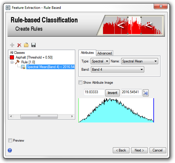
A default rule set was created when you added the new class, with one attribute: Spectral Mean(Band 1) > 169.50. You need to change this from Band 1 to Band 4. Click on the Spectral Mean attribute name, then select Band 4 from the Band drop-down list under the Attributes tab.
The cyan-colored histogram shows the frequency of Spectral Mean (Band 4) values for each segment in the segmentation image.
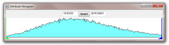
- Click the Dock/Undock Histogram Window button
 to display the histogram in a separate dialog. This option is only available for Windows users.
-
Click and drag a corner of the Attribute Histogram window to enlarge it, so that you can better view the shape of the histogram.
- Enable the Preview option in the Rule-based Classification panel. A Preview Window appears, with a solid-red color.
- Zoom out to approximately 50% using the Fixed Zoom Out button in the toolbar, so that you can view more of the image in the display.
-
Since the roads have a low spectral mean, you want to evaluate only the lowest values in the histogram. Click the blue triangle in the lower-right corner of the Attribute Histogram dialog, and drag the blue vertical bar to the left. The Preview Window will update to show the segments that remain. The following image shows an example:
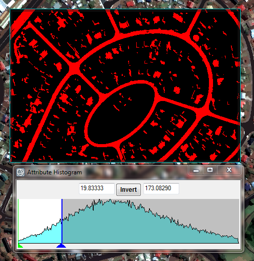
Constraining the Band 4 spectral mean values to less than 174 seems to effectively highlight the asphalt roads. (The slider only allows fractional values; type 174 into the right-most field and press Enter.)
-
Move the Preview Window to the lower-right corner of the image over the water:
-
The large red area in the right side of the Preview Window is water, which has an even lower spectral mean in Band 4 than the asphalt. So, water is also included in this histogram range. You want to exclude these extremely low values. A minimum value of 85 seems to reasonably exclude the water from consideration; type 85 into the left-most field of the Attribute Histogram dialog, and press Enter.
- Click the red X button in the Attribute Histogram dialog to close it.
- Disable the Preview check box in the Rule-based Classification panel.
Major Length Attribute
The roads and most of the parking lots in this image are lengthier than other features such as houses, so you should test one of the length attributes to see if it improves your rule set.
- In the Rule-based Classification panel, select the rule name Rule [1.0].
- Click the Add Attribute To Rule button
 .
.
- Select the default Spectral Mean(Band 1) attribute that was added.
- From the Type drop-down list, select Spatial.
- From the Name drop-down list, notice that there are three different attributes related to length: Length, Elongation, and Major Length. Select Length, and enable the Show Attribute Image option.
- Enable the Preview check box. The Preview Window displays a grayscale image of Length attribute values, with the highest values shown in white. If your feature of interest shows a high contrast (either bright or dark) relative to other features, then that attribute may be a good choice.
-
Move the Preview Window around the image. Notice how some of the roads have high Length attribute values (indicated by white), but other roads and most parking lots have lower values (indicated by gray). So this particular attribute may not effectively identify all of the asphalt.
Tip: You can check the actual attribute values for these segments by clicking the Cursor Value button  in the main toolbar. In the Cursor Value dialog, look for the "Data" line underneath Preview Window: FX_CLASSIFY_RULE_STEP. This is the Length attribute value for the segment underneath your cursor. Use these values to guide how much you want to limit the histogram.
-
Try a different length-related attribute. From the Name drop-down list, select Major Length and enable the Show Attribute Image option. More of the roads and parking lots should have a slightly higher contrast than surrounding features, compared to the Length attribute.
- Disable the Show Attribute Image check box.
- Since roads are lengthier than other features, you want to constrain the histogram to the highest Major Length values. Click the green diamond at the bottom left of the histogram, and drag the green vertical slider toward the right. Many different features are still included (shown in red) in the Preview Window. To filter out these features, you must constrain the histogram to include only extremely high values.
- Leave the maximum value as-is, but change the minimum value to 22 in the Attribute Histogram dialog, and press Enter.
- To make the next steps quicker, disable the Preview option.
Texture Mean Attribute
Asphalt roads and parking lots generally have a uniform texture, so you can experiment with the Texture attributes to see if any of them work well in extracting these features. Texture Range, Texture Mean, Texture Variance, and Texture Entropy are the four texture attributes that are calculated for every band in the image.
Prior tests show that the Texture Mean attribute for Band 4 (near-infrared) works well in identifying asphalt because it shows a high contrast in road and parking lot segments, relative to surrounding features.
- In the Rule-based Classification panel, select the rule name Rule [1.0].
- Click the Add Attribute To Rule button .
- Select the default Spectral Mean(Band 1) attribute that was added.
- From the Type drop-down list, select Texture.
- From the Band drop-down list, select Band 4.
- From the Name drop-down list, select Texture Mean.
- You want to identify segments with the lowest Texture Mean Band 4 values. A maximum value of 155 effectively identifies these segments, so enter 155 in the right-most field of the histogram and press Enter on your keyboard.
Area Attributes
So far, your rule consists of the following attributes:
- 85 < Band 4 Spectral Mean < 174, AND
- Major Length > 22, AND
- Texture Mean < 155
Next, you will use the Area attribute to filter out smaller features that remain such as shadows and rooftops.
- In the Rule-based Classification panel, select the rule name Rule [1.0].
- Click the Add Attribute To Rule button .
- Select the default Spectral Mean(1) attribute that was added.
- From the Type drop-down list, select Spatial.
- From the Name drop-down list, select Area.
- You want to identify segments with higher Area values. A minimum value of 40 effectively identifies these segments, so enter 40 in the left-most field of the histogram and press Enter on your keyboard.
Preview the Classification
Now that you have built a rule set using four different attributes, you can preview how well the rule identifies asphalt surfaces.
- In the Rule-based Classification panel, select the rule name Rule [1.0].
-
Enable the Preview option. The Preview Window shows a rule confidence image. The brightest segments have a high likelihood of satisfying the conditions of your rule, based on the attributes you selected. Dark or black features have little or no likelihood of meeting the conditions. In the following example, the roads and parking lots are bright, which means the rule set you built will most likely classify these segments as Asphalt.
-
On the left side of the Rule-based Classification panel, select All Classes. The Preview Window shows a classification image with only one class (Asphalt). This allows you to preview the final classification in a small area before classifying the entire image.
-
-
Click once inside the Preview Window, then lower its transparency using the Transparency slider in the main toolbar. This lets you preview the Asphalt class over the Region Means image.
- Click the Save Rule Set button
 in the Rule-based Classification panel.
- Select an output path and filename for the rule set. You can restore this rule file later if you want to continue where you left off.
- Click Next to proceed to the Output panel.
Specify Output Options
The Output panel lets you export various components of the rule classification to raster images and/or shapefiles. For this tutorial, you will only export a classification image of the Asphalt class to ENVI raster format, then overlay the class on the original image.
- In the Export Vector tab, disable the Export Classification Vectors option.
- In the Export Raster tab, enable the Export Classification Image option. Select an output directory to save the file to (in ENVI raster format). Change the output filename to asphalt_class.
- Click Finish. ENVI adds a new layer called asphalt_class.dat to the Layer Manager and displays it over the original GeoEye-1 image.
- Use the Pan tool to navigate around the image and evaluate the asphalt class.
The rule set did a fairly good job of extracting asphalt, but like any automated method, it did not extract every segment that represents asphalt. Some roads or parking lots were mixed with dirt, or they displayed much brighter signatures than other similar features. Successful results depend heavily on good segmentation, followed by effective rule building. If you are not satisfied with your results, try experimenting with different segmentation and merging values, or try a different set of attributes.