In this tutorial, you will use ground control points (GCPs), an orthorectified reference image, and a digital elevation model (DEM) to orthorectify an OrbView-3 scene that contains rational polynomial coefficients (RPCs).

You will learn two different methods for performing RPC orthorectification:

• Automatically generate GCPs from an orthophoto base layer, then use the GCPs in the RPC Orthorectification Workflow. This is an interactive approach that lets you assess the errors of individual GCPs as well as the overall model accuracy.
• Automatically generate GCPs and perform RPC orthorectification in one step using the RPC Orthorectification Using Reference Image tool.

Files Used in this Tutorial

Tutorial files are available from our ENVI Tutorials web page. On the ENVI Tutorials page, click the link to "ENVI Tutorial Data" to download all tutorial data. Files for this tutorial are in the rpc_ortho directory.

OrbViewSubset.dat

NAIPReferenceImage.dat

DEM.dat

Background

An RPC model is a type of sensor model that maps the physical relationship between 3D ground points and 2D image points. RPCs are not the same as a map projection. Most modern high-resolution sensors such as WorldView-3 and Pleiades include pre-computed RPCs with their imagery.

The ENVI RPC Orthorectification tools use RPCs- along with x/y/z data from GCPs and elevation data from a high-resolution DEM- to create an orthorectified image.

The reference image should have the same or slightly higher spatial resolution than the source image that you want to orthorectify. For coverage within the United States, you can obtain digital reference images from the following sources:

• U.S. Department of Agriculture National Agriculture Imagery Program (NAIP)
• U.S. Geological Survey Digital Orthophoto Quadrangles (DOQs)
• U.S. Geological Survey High-resolution Orthoimagery
• Controlled Image Base (CIB)

Download data from the U.S. Geological Survey National Map and Download Platform or EarthExplorer, then use the Seamless Mosaic tool to create a mosaic of individual tiles.

Try to choose a reference image that is close to the year and season of the input image. Automatic GCP generation is based on image matching between the reference and source images, so the scene contents should not be vastly different. Automatic GCP generation is more robust if the reference image and input image have similar resolution. If the reference image has a much higher resolution than the input image (i.e., the ratio is greater than 2.5), consider down-sampling the reference image first.

The DEM must cover at least the spatial extent of the input raster. If you do not have a DEM file readily available, you can use the Global Multi-resolution Terrain Elevation Data 2010 (GMTED2010) DEM named GMTED2010.jp2 that is provided under the ENVI installation folder. The GMTED2010 dataset has a mean resolution of 30 arc seconds. However, for best results, you should use a DEM raster with a higher resolution than GMTED2010. Many DEM products are available from the U.S. Geological Survey National Map and Download Platform or EarthExplorer.

Once you have a good-quality reference image and DEM, you can begin RPC orthorectification.

RPC Orthorectification Workflow

Open Images

1. In the toolbar, click the Open button .
2. Navigate to the directory where you saved the tutorial data. Use Ctrl-click to select the files in the following order:
   • OrbViewSubset.dat
   • NAIPReferenceImage.dat
   • DEM.dat
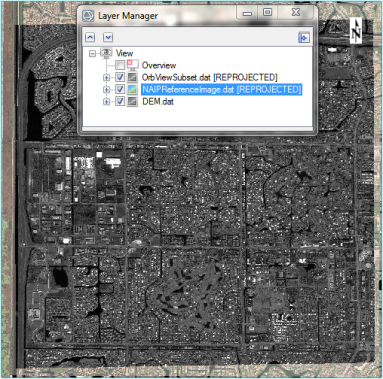
3. Click Open. The images appears in the display and are listed in the Layer Manager.
4. Right-click on the OrbViewSubset.dat layer in the Layer Manager and select View Metadata.
5. Select RPC Info in the left column of the Metadata Viewer. This field shows the RPC coefficients read from the source metadata. Verifying that an RPC Info field exists in the metadata will ensure that you can use the image with the RPC Orthorectification workflow.
6. Close the Metadata Viewer.
7. Zoom out until you can see the extent of the combined layers. The OrbView-3 panchromatic image is on top. The NAIP reference image is underneath, displayed in true color. The DEM has the same spatial extent as the NAIP image, so it is hidden beneath the other layers.
8. To increase the display area, you can click the detach icon in the Layer Manager. It becomes a floating dialog that you can move around and resize:

Create GCPs

1. In the Toolbox, expand the Geometric Correction folder and double-click Generate GCPs from Reference Image. You will use this tool to automatically create GCPs.
2. Click the Browse button next to the Input Raster field, and select the file OrbViewSubset.dat. Click OK in the Data Selection dialog.
3. Click the Browse button next to the Input Reference Raster field, and select the file NAIPReferenceImage.dat. Click OK in the Data Selection dialog.
4. Click the Browse button next to the Input DEM Raster field, and select the file DEM.dat, then click OK.
5. Leave the default value of No for DEM is Height Above Ellipsoid. The National Elevation Dataset (NED) DEM contains orthometric heights, which are elevation values above mean sea level (not above the ellipsoid).
6. Keep the default value of 25 for Requested Number of GCPs.
7. Select an output filename (with a .pts extension) and directory for the GCPs that will be created.
8. Click OK to generate the GCPs. ENVI writes the GCPs to the specified directory but does not display them. You will restore the GCPs later.

Start the RPC Orthorectification Workflow

1. In the Toolbox, expand the Geometric Correction > Orthorectification folder.
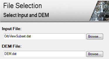
2. Double-click RPC Orthorectification Workflow. The File Selection panel appears.
3. The Input File field should already list OrbViewSubset.dat. If not, click the Browse button and select this image for input.
4. The DEM File field lists GMTED2010.jp2 as the default DEM. This global DEM provided with your ENVI installation has too coarse of a resolution for RPC orthorectification. Click the Browse button and select DEM.dat instead.



5. Under the Advanced tab, the Geoid Correction option is enabled by default. You should enable this when using DEM data containing orthometric heights (for example, GMTED2010 and NED). If you disable this option, the Horizontal Accuracy value will increase significantly. The RPC Orthorectification workflow performs geoid correction by using the Earth Gravitational Model (EGM) 1996 to automatically determine the geoid offset, which is displayed next to the Geoid Correction option.

Note: The geoid offset is the height (in meters) of the geoid above the WGS-84 ellipsoid. This constant value is added to every value in the DEM. The geoid offset accounts for the difference between the elevation above mean sea level and the height above the ellipsoid.

6. Click Next to proceed to the RPC Refinement panel.

Import GCPs

In this section, you will load the GCPs that you just created into the workflow, evaluate their horizontal and vertical accuracy, and adjust them as needed to improve the accuracy of the RPC model.

1. Click the Load GCPs button in the RPC Refinement panel.
2. Navigate to the directory where you saved the GCP file (.pts), and select it. Click Open. The GCPs appear as green crosshairs in the image display, and they are listed in the RPC Refinement panel as follows:



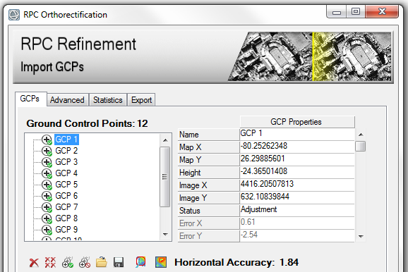
Even though you requested 25 GCPs in the Generate GCPs from Reference Image tool, it only created 12 GCPs. During the GCP generation process, ENVI first creates tie points between the OrbView-3 and reference images. It then filters the tie points for radiometric and geometric quality. It creates GCPs from the remaining tie points.

This panel provides some basic details about the GCPs:

• The green check marks indicate that these GCPs are active and will be used to adjust the RPC model. These points are called adjustment GCPs.
• When you select a GCP in the list, the details of the GCP location appear in the GCP Properties table to the right. Included are the longitude and latitude in a Geographic Lat/Lon WGS-84 projection; height in meters above the WGS-84 ellipsoid; image coordinates; status (adjustment or independent); and error statistics. The next section will discuss the error statistics in more detail.
• The Horizontal Accuracy value is the horizontal root mean square error (RMSE) in meters. In the example above, all of the adjustment GCPs taken together would yield an orthorectified image that is accurate to within 1.84 meters. In the next section, you will try to increase its accuracy.

View Errors

Here, you will assess the quality of your GCPs and how they contribute to the overall accuracy of the orthorectification. Once you identify GCPs with large errors, you can adjust them or delete them, then re-evaluate the accuracy of the orthorectification.

Rather than give a mathematical definition of all of the available error statistics, this tutorial will highlight the most important ones to evaluate and will give you a more practical approach to understanding their meaning. For details, see Accuracy Assessment Background.

1. Right-click on the OrbViewSubset.dat layer in the Layer Manager, and select Zoom to Layer Extent.
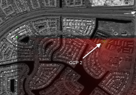
2. In the RPC Refinement panel, click the Show error overlay button . A transparent image overlays the scene, showing a color gradient of interpolated GCP errors. The darkest areas indicate GCPs with the least error, and the bright red areas indicate GCPs with higher errors.

The error overlay should look similar to the following image:



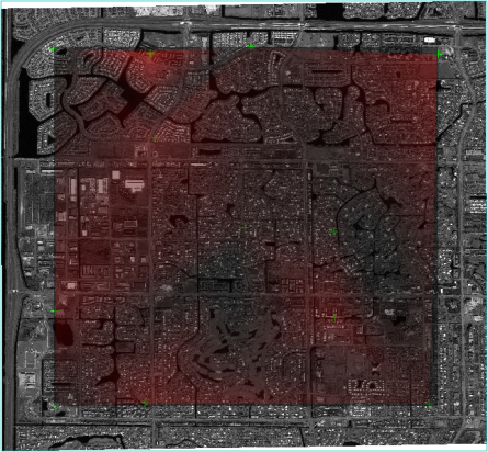
The error overlay is useful for quickly evaluating how the GCP errors are distributed across the entire image. Use the Zoom and Pan tools in the main toolbar to explore the image in more detail if needed.

3. Click on each GCP in the list, then scroll down in the GCP Properties table to see its Error Magnitude value. GCP 2 has the highest value at 3.81 meters. This GCP is located at the top of the image and corresponds to the brightest area of the error overlay:



4. In the RPC Refinement panel, click the Hide error overlay button to turn off the error overlay.

Correct Errors

If more accurate geolocation information is available for a given GCP, you can edit its Map X and Map Y values in the GCP Properties table. You can also experiment with different Image X and Image Y values. However, in most cases, it is more practical to interactively move the GCP location in the image display, then re-evaluate its error statistics. Or, delete a GCP if moving its location does not improve the error statistics.

1. Select GCP 2 in the list, then click the Delete button . The Horizontal Accuracy value slightly improves to 1.41 meters.
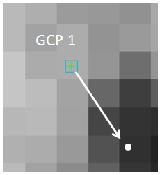
2. Again, click on each GCP in the list, then scroll down in the GCP Properties table to see its Error Magnitude value. GCP 1 now has the highest Error Magnitude value at 2.42 meters.
3. With GCP 1 centered in the display, use the Zoom tools to zoom into the OrbView-3 image until the pixels appear blocky.
4. With the Select icon active in the main toolbar, click and drag the GCP 1 marker a few pixels to the southeast:



The Horizontal Accuracy value improves to approximately 1.05.

5. Continue this process until the Horizontal Accuracy value is less than 1 meter. Adjusting too many GCP locations may actually introduce more error; two or three GCPs will suffice.

Vertical Accuracy

Elevation data significantly improves the accuracy of RPC orthorectification, so that is why a digital elevation model (DEM) is required for input. The RPC Orthorectification workflow uses elevation data in conjunction with geolocation data to compute an RPC solution. Various statistics are available for you to evaluate the vertical accuracy of the model.

Select the Statistics tab. The RMSE Z value is the root mean square of the Error Z values for the entire image. It reports the vertical accuracy of the entire RPC model. The LE95 value is the difference (in meters) between the GCP-measured elevation and the DEM elevation, using the calculated geoid offset at the 95% confidence level.

Save GCPs to a Shapefile

Once you are satisfied with the quality of your GCPs, click the Save GCPs button under the
GCPs tab in the RPC Refinement panel. Select an output shapefile name and location. If you quit the workflow, you can continue where you left off by re-loading the input image, DEM, and new GCP shapefile.

Now that you have reduced the individual GCP errors and the overall model error, you can preview the orthorectification in a limited area before orthorectifying the entire image.

Orthorectify the Image

1. Click the Advanced tab. Notice that the Output Coordinate System for the orthorectified result will be UTM Zone 17N by default.
2. Click the Export tab. Choose a directory where you want to create the orthorectified image.
3. Enable the Export Orthorectification Report option, and choose a directory for the output report. This report will list the source files used, adjustment and independent GCPs, geoid offset, error statistics, and output settings.
4. Click Finish to generate the orthorectified image. When processing is complete, the RPC Refinement panel closes, and the orthorectified image is displayed and added to the Layer Manager. It will have some black background pixels along the edge because of the reprojection that took place.
5. In the Layer Manager, toggle the orthorectified image on and off to compare it to the original OrbView-3 image.
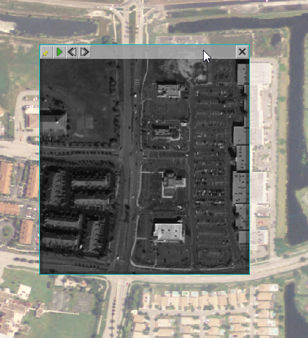
6. Compare the orthorectified image to the NAIP reference image. The location of roads and buildings should match between the two layers. The following example shows a Portal with the orthorectified result overlaid on the NAIP reference image:



7. In the Layer Manager, right-click on all layers except NAIPReferenceImage.dat and select Remove.

Automated RPC Orthorectification

Instead of using the RPC Orthorectification workflow, you can use the RPC Orthorectification Using Reference Image tool to quickly orthorectify an RPC image. It automatically generates GCPs using a reference image and DEM before orthorectifying the image. This tool is useful when you want a more automated approach to generating GCPs without checking their RMSE values. Follow these steps:

1. Display the NAIPReferenceImage.dat image. You will compare the orthorectified image to this reference image later.
2. In the Toolbox, expand the Geometric Correction > Orthorectification folder, and double-click RPC Orthorectification Using Reference Image.
3. Click the Browse button next to the Input Raster field, and select the file OrbViewSubset.dat, then click OK,
4. Click the Browse button next to the Input Reference Raster field, and select the file NAIPReferenceImage.dat, then click OK.
5. Click the Browse button next to the Input DEM Raster field, and select the file DEM.dat, then click OK.
6. Leave the default value of No for DEM is Height Above Ellipsoid.
7. Increase the Requested Number of GCPs to 40.
8. Leave the default value of Bilinear for the Resampling Method.
9. Leave the default value of 10 for Grid Spacing.
10. Enter an output filename and directory for the orthorectified raster.
11. Enter an output filename (.pts) and directory for the output GCPs.
12. Enable the Display result option.
13. Click OK. When processing is complete, toggle the orthorectified image on and off to compare it to the underlying reference image.
14. Repeat this process and experiment with different values for Requested Number of GCPs to achieve the desired result.
15. When you are finished examining the images, close ENVI.