Raster layers generally refer to images, including multispectral, panchromatic, digital elevation models (DEMs), and masks. For information about classification images, see Class Layers.
See the following sections for details on raster layers:
Working with Raster Layers
The Layer Manager lists all of the displayed files in a tree view. Raster layers that are open but are not displayed in a view will be listed in the Data Manager.
Each time you open a new raster file, the layer is added to the top of the Layer Manager tree and it becomes the selected layer. The selected layer is what you can perform specific functions on (such as add ROIs), without affecting other layers.
Here are some general tips for working with layers:
- To select a layer, click its name in the Layer Manager.
- Basic metadata for the selected layer (such as Name) displays in the Layer tab, located below the Toolbox.
- To remove a layer from the view, right-click and select Remove. Removing a layer from the Layer Manager tree will remove it from the view, but the file will remain open in the Data Manager.
- To select multiple layers, use Ctrl+click or Shift+click and select the desired layers. To perform actions on the selected layers, right-clicking and select an option from the context menu.
- To hide a single layer in a view, disable the check box for that layer in the Layer Manager. To show the layer, enable the check box.
- To hide selected layers in the view, use Ctrl+click to multi-select the layers to hide, then right-click and select Hide All Layers. To show selected layers that are hidden, use Ctrl+click to multi-select the layers to show, then right-click and select Show All Layers.
- To hide all layers in a view, right-click on the View icon in the Layer Manager and select Hide All Layers. To show all layers, right-click and select Show All Layers.
- If you created multiple views in the Image window, the layers for each view are grouped under View entries.
- If you have multiple views displayed, you can drag-and-drop layers from the Layer Manager to any one of those views in the display or to the corresponding view icons in the Layer Manager. This creates a copy of the layer(s) to populate the views.
- You can dynamically change the band selection that was automatically loaded when the file was opened.
- If a raster has bad bands defined in the header file, those bands are marked with a warning symbol in the Layer Manager.
- Drag-and-drop individual ROI layers or ROI containers from one raster to another, to load the selected ROIs in the new raster layer.
- To add a band to a new view, select the filename in the Data Manager, then select the band to load. Enable the Load in New View check box, then click Load Data.
Manage Individual Layers
For additional options with individual layers, right-click on a raster in the Layer Manager and select an option:
- Rename Item: Enter the new name in the Rename Item dialog and press the Enter key to accept it or press the Esc key to cancel. (Linux and Mac users should click the green check icon to accept the new name or click the red X icon to cancel.)
- Export Layer to TIFF: Save the full raster layer extent, with image enhancements, at full resolution to a TIFF file.
- Display in Portal: Display the raster layer in a portal.
- Order: Change the order in which a layer is displayed relative to other layers. Choose one of the following options:
- Bring to Front
- Bring Forward
- Send Backward
- Send to Back
Or, select a layer and drag it to the desired order in the Layer Manager.
-
Remove: Remove the layer from the Layer Manager. The file remains open and you can access it and redisplay it from the Data Manager.
- New Region of Interest: Create a new ROI layer for the selected raster.
- New Raster Color Slice: Create a new color slice layer for the selected raster.
- New Contour Layer: Create a new contour layer for the selected raster.
- Band Animation: Animate through the bands of a raster using the Xtreme Viewer or as a Raster Series.
- Change Color Table: Change the color table for a grayscale raster. This menu option is not available for single-band layers that contain predefined color palettes, such as ENVI classification images. Choose one of the following predefined color tables:
- Greyscale
- Blue/White
- Red Temperature
- Blue/Green/Red/Yellow
- Rainbow
Or, select More to use the ENVI Color Table dialog to create your own color table.
- Profiles: Create plots of spectral, horizontal, vertical, arbitrary, and series profiles.
- View Metadata: Open the View Metadata dialog for a raster layer. Basic metadata properties are also displayed in the lower-right corner of the ENVI application without requiring you to select this menu option.
- Quick Stats: Compute basic statistics and histograms for all bands.
- Zoom to Layer Extent: Center and display the entire layer within a view.
- Zoom to Layer Full Resolution: Zoom to 1:1 (100%) scale.
Selecting Full Extent from the Zoom drop-down menu or clicking the Zoom to Full Extent button  in the main toolbar zooms to the combined extents of all layers for the current view. Also, if a raster layer is georeferenced, the Zoom To drop-down list in the main toolbar displays options for Use Map Scale and Use Pixel Scale. For pixel-based raster layers (with no georeferencing), the Zoom To drop-down list only displays options for Use Pixel Scale.
- If you open an OGC WMS raster layer that contains a legend, the legend displays in the Layer Manager. To create an annotation object from the legend that you can overlay on the image, right-click the layer name and select Load Layer as Annotation. This is useful, for example, in creating a Powerpoint presentation from the view.
- Load Current Raster: Load the current raster in a series as a separate layer. This option is only available for raster series data.
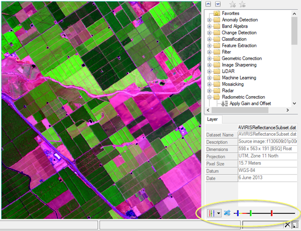
Change Band Selection
ENVI uses information from the image metadata to determine what RGB band combination to load when the opens in the view. You can use the Dynamic Band Selection tool to change this initial band selection after the raster has been loaded. The tool is available at the bottom of the Layer tab whenever a raster is the selected layer in the Layer Manager.
This section describes how to use the Dynamic Band Selection tool to do the following:
- Select preset band combinations from a list
- Select your own band combinations
- Let ENVI select random band combinations for you
- Save band combinations to reuse or share
For the band selection options listed above, you can easily change the combinations as often as desired to see the new combinations automatically applied in the view.
Select a Preset Band Combination
ENVI provides several preset band combinations you can apply. If you save custom band combinations, they also appear in the list of presets. Click the drop-down arrow next to the sliders  and make a selection. ENVI provides the following:
- True Color
- Color Infrared
- Shortwave Infrared
- False Color
- Agriculture
- Vegetation
- Geology
- Bathymetric
- Atmospheric Penetration
- Land/Water
Select Your Own Band Combinations
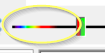
To make your own band combinations, click and drag the slider bars for red, blue, and green to select the bands to use for each.
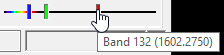
The visible light, and what the wavelengths are for visible light, are shown on the left side of the slider bar.
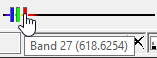
Select Random Band Combinations
To have ENVI randomly select band combinations, click the Select Random Band Combination button  .
.
Save Band Combinations
You can save band combinations you created or that ENVI randomly selected for you. Saved RGB band combinations are added to the drop-down list of presets. The band combinations are also saved to the file .idl\envi\preferencesx_x\display_bands.json, which can be shared with other ENVI users.
To save band combinations:
- Click the drop-down arrow next to the sliders and select Add Band Combination.
- Enter a Band combination name or use the default name, then click the OK
 button to save.
To remove saved band combinations from the drop-down list and the display_bands.json file, click the drop-down arrow and select Reset Band Combinations.
To restore band combinations from a file, click the drop-down arrow and select Restore Band Combinations, then browse and select the display_bands.json file.
Hybrid Band Selection in the Data Manager
You can create a new RGB layer consisting of three bands from different files, see Data Manager for details. The images must be coregistered and have the same x and y dimensions. Bands from a palette-based image are not supported.
Change a Color Table
To apply a color table to a grayscale image, right-click the layer in the Layer Manager and select Change Color Table, then select the color table to apply from a short list of predefined IDL color tables. Or, for additional options, select More, then click the Edit Color Table button  . In the Edit Table Color dialog that appears, you can choose from the complete list of predefined IDL color tables, define a color gradient, or work with different color spaces. See Edit Color Tables for details.
Change Interpolation
You can change the interpolation method to use on a raster layer or raster series layers. Interpolation behavior may vary, depending on the method you choose, and whether the Use Graphics Card to Accelerate Enhancement Tools preference is enabled. Variations are noted in the following descriptions. The choices are as follows:
- Nearest Neighbor: Each pixel in the displayed image receives its value from the nearest pixel in the input (reference) image. If the Use Graphics Card to Accelerate Enhancement Tools preference is enabled, brightness, contrast, and sharpen filters are performed by the GPU.
- Bilinear: Each estimated pixel value in the displayed image is based on a weighted average of the four nearest neighboring pixels in the input image.
Not all GPUs support bilinear interpolation of floating point textures; therefore, if Use Graphics Card to Accelerate Enhancement Tools is enabled, the setting is ignored and brightness, contrast, and sharpen filters are performed by the CPU.
- Bicubic: Each estimated pixel value in the displayed image is based on a weighted average of the sixteen nearest pixels in the input image. If Use Graphics Card to Accelerate Enhancement Tools is enabled, the setting is ignored and brightness, contrast, and sharpen filters are performed by the CPU. If your graphics processing unit (GPU) does not support OpenGL Shader Language (GLSL), the Nearest Neighbor interpolation method is used instead.
- Optimized Bicubic: (default) Each estimated pixel value in the displayed image is based on a weighted average of the sixteen nearest pixels in the input image. The weighting coefficients are improved over standard Bicubic. If Use Graphics Card to Accelerate Enhancement Tools is enabled, the setting is ignored and brightness, contrast, and sharpen filters are performed by the CPU. If your graphics processing unit (GPU) does not support OpenGL Shader Language (GLSL), the Nearest Neighbor interpolation method is used instead.
To use Bicubic and Optimized Bicubic:
- Your graphics card must support OpenGL 2.0 or higher, and you must have the most recent drivers installed.
- ROIs will always display as Nearest Neighbor, regardless of the preference setting.
Portals behave differently; they try to match the interpolation value of the target layer, regardless of the current preference setting.
Send Files to ArcGIS Pro
If ArcGIS Pro is installed, you can send one or more open files from ENVI to ArcGIS Pro. When the dataset displayed in both ENVI and ArcGIS Pro, you can set the extent to use, and link the ENVI view and ArcGIS Pro view to synchronize them. See ArcGIS Pro Integration for details on setting extents and linking the views.
Supported file types are rasters and vectors. Raster files must be saved in a format supported by ArcGIS Pro. If ArcGIS Pro cannot read the file, ENVI will save the raster to a .dat file before sending it to ArcGIS Pro.
Note that ArcGIS Pro uses different logic to open raster files in terms of histogram stretching and how to handle files that produce multiple rasters when opened (such as NITF). This is due to ENVI not sending pixel data to ArcGIS Pro, it is sending a file to open.
To send files to ArcGIS Pro from the Layer Manager:
- Start ArcGIS Pro.
- Select the file(s) to send in the Layer Manager, then right-click and select Send to ArcGIS Pro.
- ArcGIS Pro creates a project for the dataset, then opens it in a view.
View and Edit Metadata
You can view the metadata in the header file, and you can add and edit header file fields.
-
To view metadata, right-click on the layer name in the Layer Manager and select View Metadata. See View Metadata for details.
-
For descriptions of the metadata fields, see ENVI Header Fields.
-
To add or edit metadata in the header file, see Edit ENVI Headers.
See Also
Supported Data Types, Data Manager, ENVI Header Files, Contour Layers, Raster Color Slices, Edit Color Tables