This tutorial uses EO-1 Hyperion hyperspectral imagery to identify areas of dying conifers resulting from insect damage. You will learn how to pre-process the imagery and how to create vegetation indices that exploit specific wavelength ranges to highlight areas of stressed vegetation.
See the following sections:
Files Used in this Tutorial
Tutorial files are available from our ENVI Tutorials web page. Click the Hyperspectral link to download the .zip file to your machine, then unzip the files. You will use this file for the tutorial:
|
File |
Description |
|
HyperionForest.dat
|
EO-1 Hyperion image in ENVI raster format with 242 spectral bands at 30 m spatial resolution, acquired on 20 July 2013.
|
The gray polygon in the following map shows the approximate coverage area of the image. It covers a small area of St. Joe and Clearwater National Forests in eastern Idaho, USA.
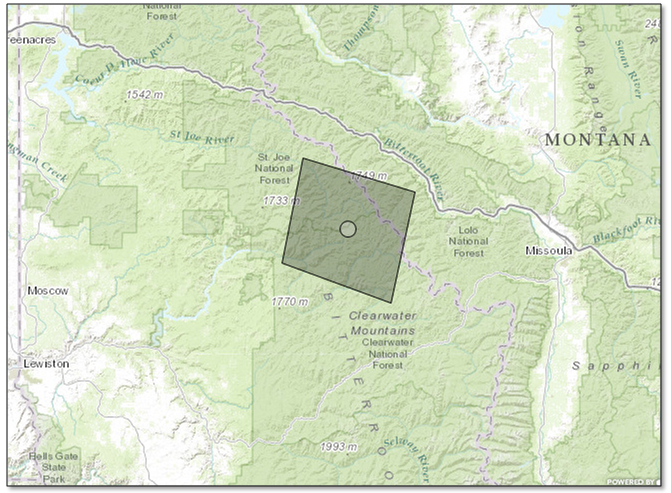
This particular Hyperion scene was chosen for the tutorial because it shows evidence of widespread insect damage from the Mountain Pine Beetle and Western Balsam Bark Beetle.
Preprocessing
Follow these preprocessing steps before doing any scientific image analysis.
Open and Display the Image
- From the ENVI menu bar, select File > Open.
- Select the file HyperionForest.dat. Click Open.
This image is a spatial subset of a larger Hyperion image, which was downloaded from the USGS EarthExplorer web site in HDF4 (Level-1R) format. We defined a spatial subset and saved it to ENVI raster format to create a smaller file for this tutorial. We also shortened the band names in the associated header file.
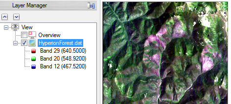
If the Auto Display Method for Multispectral Files preference is set to True Color, the image is displayed using bands 29 (red), 20 (green), and 12 (blue) to yield an approximate true-color representation:
- Press the F12 key on your keyboard to view the image at full extent.
- Explore the image in more detail using the navigation tools in the toolbar. In a true-color display, dead and stressed vegetation is colored gray or red-gray. Beetle damage is likely responsible for the dying conifers in this region. Healthy vegetation is colored green.
View Metadata
- In the Layer Manager, right-click on the filename HyperionForest.dat and select View Metadata. The View Metadata dialog appears.
- Click on the Coordinate System category. The coordinate system of the image is Geographic Lat/Lon WGS-84, but that does not mean the image is correctly georeferenced.
- Click on the Geo Points category. The Geo Points category indicates that only the four corner points of the image are known. ENVI treats this as a pseudo projection. It applies an affine map transformation to warp the image based on the four corner points and Kx/Ky coefficients. It attempts to calculate geographic coordinates for each pixel. This type of projection contains a high degree of variability and is not geographically accurate. ENVI does not have tools to orthorectify Hyperion data. One option is to use the Image to Map Registration tool to create ground control points for image-to-map registration, though this tutorial will not cover these steps.
- Close the View Metadata dialog.
Correct for Atmospheric Effects
Calibrating the imagery to apparent surface reflectance yields the most accurate results when using spectral indices. This is especially important for hyperspectral sensors such as AVIRIS and EO-1 Hyperion. Calibrating imagery to surface reflectance also ensures consistency when comparing indices over time and from different sensors.
If you have the separate license for the Atmospheric Correction Module: FLAASH and QUAC module you can use FLAASH in these next steps to remove atmospheric effects from the image and to create an apparent surface reflectance image.
FLAASH is a model-based radiative transfer program developed by Spectral Sciences, Inc. It uses MODTRAN6 radiation transfer code to correct images for atmospheric water vapor, oxygen, carbon dioxide, methane, ozone absorption, and molecular and aerosol scattering.
Follow these steps:
- In the Toolbox, type flaash. Double-click the FLAASH Atmospheric Correction tool name that appears. The Data Selection dialog appears.
- Select HyperionForest.dat and click OK. The FLAASH - Rigorous Atmospheric Correction dialog appears, with the Main tab selected.
Define Acquisition Time and Output Files
-
The Acquisition Date/Time fields should automatically populate with metadata information and should show 20 July 2013 and 17:36:52
-
In the Output Water Raster field, type the full path of the directory where you want to write the output column water vapor image. For the filename, enterSurfaceReflectance_water.
-
In the Output Raster field, type the full path of the directory where you want to write the output reflectance file. For the filename, type SurfaceReflectance.dat.
-
Disable the Display result check box for the output raster.
Sensor and Geometric Settings
- Select the Sensor tab. If available in the metadata, FLAASH will populate the Sensor Type field with the correct sensor. It should be Hyperion.
- Leave the Input Scale value at the default of 10.000.
- Set the Instantaneous Field of View to 0.1.
-
Select the Geometric tab. FLAASH automatically determines the scene's center geographic coordinates, so you do not need to enter these values. The following fields should also populate with the following metadata information:
- Sensor Altitude should be 705 for the EO-1 spacecraft
- Ground Elevation should be 1.685
Atmospheric Model, Water and Aerosol Settings
Hyperspectral sensors typically include enough information needed to estimate water vapor and aerosols in the atmosphere. You will retrieve water vapor and aerosols in the steps below.
- Select the Model tab. From the Atmospheric Model drop-down list, select 1976 US Standard Atmosphere.
- Select the Water tab. From the Water Absorption Wavelength drop-down list, select 1130.
- Select the Aerosol tab. From the Aerosol Model drop-down list, select High-Visibility Rural. This is a good option for the location of the scene, where aerosols are not strongly affected by urban or industrial sources. The choice of model actually is not critical in this case, as the visibility is typically greater than 40 km.
- Click OK. FLAASH processing may take several minutes. FLAASH creates several output files in the directory that you defined: a cloud mask image, water vapor image, and the reflectance file.
Display the Reflectance Image
- Click the Data Manager button
 in the toolbar.
-
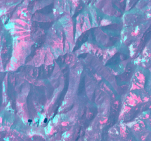
Right-click SurfaceReflectance.dat and select Load CIR. [1]SurfaceReflectance.dat is added to the Layer Manager and it displays in a false-color combination. The following figure shows an example of the northern part of the image:
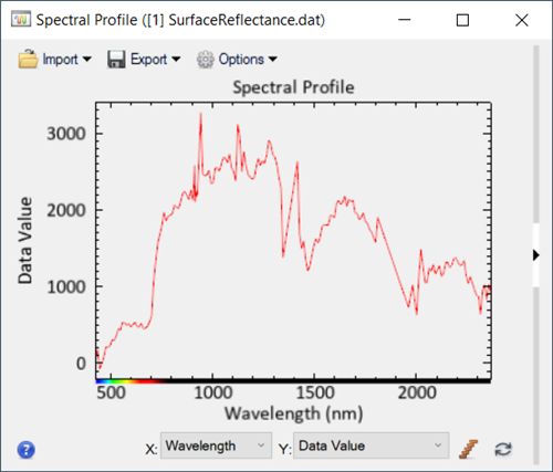
- Click the Spectral Profile button
 in the toolbar.
-
In the Go To field in the toolbar, enter the following pixel coordinates: 10, 762. This pixel represents healthy vegetation. Note the shape of the reflectance curve with the abrupt increase in reflectance from 680 to 730 nm (referred to as the red edge). This wavelength region is often analyzed in more detail when studying factors that stress vegetation. Two strong absorption features representing vegetation water content are evident at 1450 nm and 1950 nm. You can also see a peak in the green wavelength region near 550 nm.
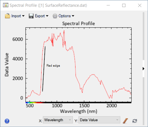
In the Go To field in the toolbar, enter the following pixel coordinates: 227, 342. This location contains unhealthy conifer trees. Note the shape of the reflectance curve. In general, the slope of the red edge has decreased significantly and the 1450 nm water absorption feature is not as prominent, indicating lower moisture content.
- Close the Spectral Profile in preparation for the next exercise.
While spectral profiles can help locate pixels with unhealthy vegetation, spectral indices can give us a more accurate assessment of stressed vegetation.
Vegetation Indices
Spectral indices are combinations of surface reflectance at two or more wavelengths that indicate relative abundance of features of interest. Vegetation indices derived from satellite images are one of the primary information sources for monitoring vegetation conditions. Detection of vegetation stress by remote sensing techniques is based on the assumption that stress factors interfere with photosynthesis or the physical structure of the vegetation and affect the absorption of light energy and thus alter the reflectance spectrum of vegetation (Riley, 1989; Pinter and Hatfield, 2003).
The spectral resolution of Hyperion imagery allows you to examine the red-NIR spectrum in more detail, which helps to identify areas of stressed vegetation. ENVI offers several narrowband vegetation indices, which indicate the overall amount and quality of photosynthetic material and moisture content in vegetation.
Follow these steps to create different vegetation indices:
- In the Toolbox, expand the Band Algebra folder.
- Double-click the Spectral Indices tool. The Data Selection dialog appears.
- The Input Raster field should already list SurfaceReflectance.dat. If not, click the Browse button and locate this file.
- Click OK. The Spectral Indices dialog appears.
- In the Index list, select Moisture Stress Index.
- In the Output Raster field, select the File radio button and name the output file MSI.dat.
- Enable the Display result check box, and click OK to create the Moisture Stress Index image.
-
When processing is complete, explore the Moisture Stress Index image in more detail. Spectral indices do not provide exact, quantitative measures of spectral properties; they only provide a relative abundance of a feature of interest. Brighter pixel values indicate more water deficiency. The Moisture Stress Index is a reflectance measurement that is sensitive to increasing leaf water content. As the water content in vegetation increases, the strength of the absorption around 1599 nm increases. Absorption at 819 nm is nearly unaffected by changing water content, so it is used as the reference wavelength (Hunt, Jr. and Rock, 1989):
White et al (2007) found significant correlation between Moisture Stress Index values and levels of pine beetle damage.
Next, you will create a raster color slice that highlights the highest pixel values in the MSI image.
Color Slices
- Right-click on the MSI.dat layer in the Layer Manager and select New Raster Color Slice. The Data Selection Dialog appears.
- Select the Moisture Stress Index band name, and click OK. The Edit Raster Color Slices dialog appears.
- Click the Clear Color Slices button
 . You will create a new raster color slice instead.
- Click the Add Color Slice button
 . A new color slice is added that covers the entire range of pixel values. Next, you will highlight the highest pixel values, which correspond to the end of the narrow histogram that is displayed.
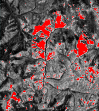
- Enter a value of 1 in the Slice Min column and keep the Slice Max value as-is.
- Press Enter key on the keyboard to set the values. Moisture Stress Index values above 1.0 are highlighted in red, for example:
- Right-click on the Slices folder in the Layer Manager and select Export Color Slices > Shapefile.
- Enter an output filename of HighMSI.shp, and click OK.
- Click OK to exit the Edit Raster Color Slices dialog.
- If the MSI.dat layer was added to the Layer Manager, uncheck the layer to hide it. The red raster color slice is displayed on top of the original surface reflectance image.
- Select the Raster Color Slice layer in the Layer Manager, then adjust the Transparency slider in the toolbar to see through the color slice to the surface reflectance image underneath.
- Uncheck the Raster Color Slice layer to hide it.
Next, you will use the Forest Health tool to look for areas with high stress conditions.
Forest Health Tool
The Forest Health Classification tool will create a spatial map that shows the overall health and vigor of a forested region. It is good at detecting pest and blight conditions in a forest as well as assessing areas of timber harvest. A forest under high stress conditions shows signs of dry or dying plant material, very dense or very sparse canopy, and inefficient light use. The tool uses the following vegetation index categories:
-
Broadband and narrowband greenness, to show the distribution of green vegetation.
-
Leaf pigments, to show the concentration of carotenoids and anthocyanin pigments for stress levels.
-
Canopy water content, to show the concentration of water.
-
Light use efficiency, to show forest growth rate.
Follow these steps to create a forest health map:
- In the search window of the Toolbox, type forest.
- Double-click the Forest Health Analysis tool name that appears. The Forest Health Classification dialog appears.
- In the Input Raster field, click the Browse button
 . The Data Selection dialog appears.
- Select the SurfaceReflectance.dat file, then click OK.
- From the Greenness Index drop-down list, select Modified Red Edge Normalized Difference Vegetation Index.
- Leave the Min Valid Greenness Value setting at 0.00.
- From the Leaf Pigment Index drop-down list, select Carotenoid Reflectance Index 2.
- From the Canopy Water or Light Use Efficiency Index drop-down list, select Structure Insensitive Pigment Index.
- Enter an Output Raster filename of ForestHealth.dat.
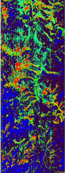
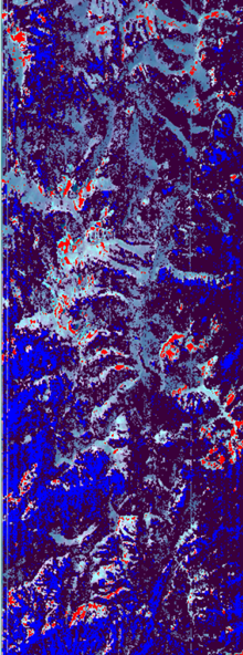
- Enable the Display result option and click OK. The Forest Health image does not provide any quantitative measures of vegetation stress; instead, it shows the relative amounts of forest vegetation health from 1 (unhealthy) to 9 (healthy). You can see the vertical striping artifacts from the Hyperion sensor.
-
In the Layer Manager, uncheck the [1]SurfaceReflectance.dat layer to hide it and uncheck all classes except for 1 and 2 under the Forest Health Classes folder:
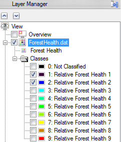
-
These pixels represent areas with stressed vegetation. Compare this with the vegetation index images you created earlier.
Field studies and aerial surveys are further needed to validate whether the areas correspond with insect damage. However, the methods that you learned in this tutorial show that remote sensing and hyperspectral imagery are effective tools for indicating unhealthy and dying vegetation in forests.
References:
Barry, P. EO-1/Hyperion Science Data User’s Guide. Redondo Beach, CA: TRW Space, Defense & Informations Systems (2001).
Ceccato, P. et al. "Detecting vegetation leaf water content using reflectance in the optical domain." Remote Sensing of Environment 77 (2001): 22-33.
Datt, B. et al. "Preprocessing EO-1 Hyperion hyperspectral data to support the application of agricultural indexes." IEEE Transactions on Geoscience and Remote Sensing 41, No. 6 (2003): 1246-1259.
Datt, B. "A new reflectance index for remote sensing of chlorophyll content in higher plants: tests using Eucalyptus leaves." Journal of Plant Physiology 154 (1999): 30-36.
Hunt Jr., E., and B. Rock. "Detection of changes in leaf water content using near- and middle-infrared reflectances." Remote Sensing of Environment 30 (1989): 43-54.
Merzlyak, J. et al. "Non-destructive optical detection of pigment changes during leaf senescence and fruit ripening." Physiologia Plantarum 106 (1999): 135-141.
Pinter, P., and J. Hatfield. "Remote sensing for crop management." Photogrammetric Engineering & Remote Sensing 69, Vol. 6 (2003): 647-664.
Riley, J. "Remote sensing in entomology." Annual Review of Entomology 34 (1989): 247-271.
Sims, D., and J. Gamon. "Relationships between leaf pigment content and spectral reflectance across a wide range of species, leaf structures and developmental stages." Remote Sensing of Environment 81 (2002): 337-354.
White, J. et al. "Detecting mountain pine beetle red attack damage with EO-1 Hyperion moisture indices." International Journal of Remote Sensing 28, Issue 10 (2007): 2111-2121.