Getting Started with ENVI Tutorial
This tutorial provides a comprehensive introduction to using ENVI. It is designed for new ENVI users or those who have used ENVI Classic in the past and want to learn the newer ENVI user interface. You will learn how to display and navigate imagery, analyze raster data, create presentations, and more.
See the following sections:
Files Used in This Tutorial
Tutorial files are available from our ENVI Tutorials web page. Click the High Resolution Ortho Photo link to download the .zip file to your machine, then unzip the files. You will use this files in the tutorial:
|
File |
Description |
|
CentralParkOrthophoto.dat (and .hdr)
|
Orthorectified digital photograph of Central Park, New York City, USA, in ENVI raster format
|
|
CentralParkWaterROI.xml
|
Region of interest (ROI) file containing polygons that identify ponds in the orthophoto
|
The digital photograph is a public-domain U.S. Geological Survey (USGS) High Resolution Orthoimage downloaded from the USGS EarthExplorer web site. Gridded spatial resolution is 0.15 meters (0.5 feet). The image contains four bands (red, green, blue, near-infrared) and was acquired between April and May of 2014.
Technical Notes
The orthophoto was originally acquired from an UltraCam Eagle digital camera, which has the following wavelength ranges for visible to near-infrared bands:
- Blue: 400 - 600 nm, peak at 450 nm
- Green: 480 - 700 nm, peak at 550 nm
- Red: 580 - 720 nm, peak at 640 nm
- Near-infrared: 680 - 1000 nm
Reference: Gruber, M., and M. Muick. "UltraCam Eagle Prime Aerial Sensor Calibration and Validation." Vexcel Imaging GmbH (2016).
The orthophoto did not have any wavelength information, so we manually added the peak wavelengths for each band to the ENVI header file. For the near-infrared band, we used the center wavelength (840 nm).
Explore an Image
- Start ENVI.
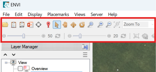
- Click the Open button
 in the toolbar. The toolbar is located along the top of the ENVI application:
- When the Open dialog appears, navigate to the location where you saved the tutorial data. Select CentralParkOrthophoto.dat and click Open. The center of the image is displayed at full (100%) resolution in the view.
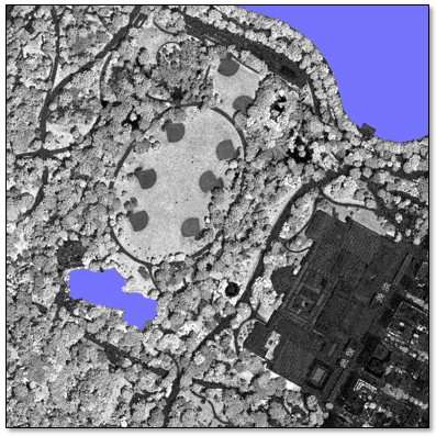
- Press the F12 key on your keyboard to view the full extent of the image. This is a true-color image that shows natural and man-made features.
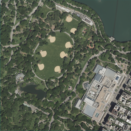
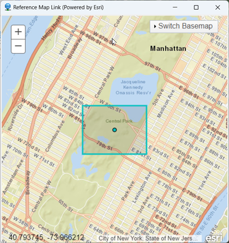
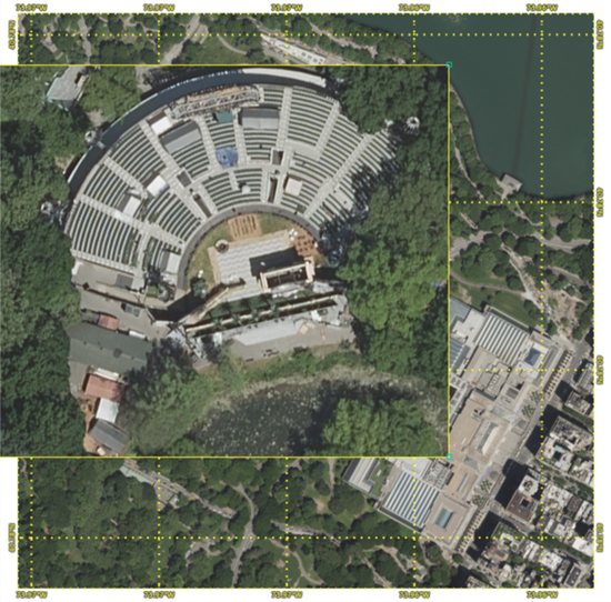
- From the menu bar (located above the toolbar), select Views > Reference Map Link. A separate window appears with a map of the image location. The cyan-colored box indicates the extent of the image, and the dot in the middle indicates the image center. You can see that the image covers a portion of Central Park in New York City. It contains several softball fields, ponds, and an amphitheater. The large building in the lower-right corner is the Metropolitan Museum.
- Explore the image using these techniques:
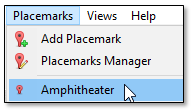
- Zoom to an area that you are interested in, then select Placemarks > Add Placemark from the menu bar.
- In the New Placemark dialog, enter a name for the location and click OK; for example:
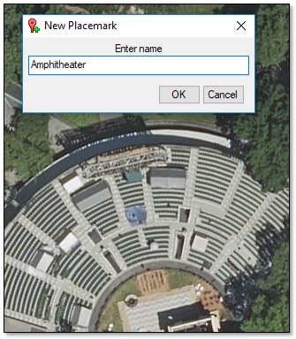
The custom location is saved under the Placemarks menu. When you move to another area in the image, you can go back to the saved location by clicking Placemarks and selecting it from the list; for example:
As you move the cursor around the image, the latitude and longitude coordinates of the cursor location are displayed in the Status Bar at the bottom of the ENVI application. The Status Bar contains three horizontal segments. By default, the first (left) segment displays geographic coordinates, and the second segment displays the map projection details for the image. The third segment is blank. The following figure shows an example of the first two segments:
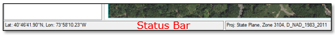
You can choose to display different types of image information in each segment by right-clicking and selecting an option.
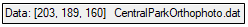
- Right-click in the first (left) segment and select Raster Data Values. The red, green, and blue data values are displayed for the current pixel location; for example:
- Zoom to full resolution (100%) in the image, then click the Overview check box in the Layer Manager. The Layer Manager is located near the upper-left corner of the application. A small yellow overview window is displayed in the upper-left corner of the view.
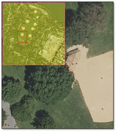
- Pan around the image. The red box in the overview window shows the extent of the current view location, relative to the entire image.
- Uncheck the Overview option to hide the overview window.
Now that you understand some basic exploration techniques, you will learn how to work with multiple data layers and views.
Work with Layers and Views
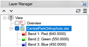
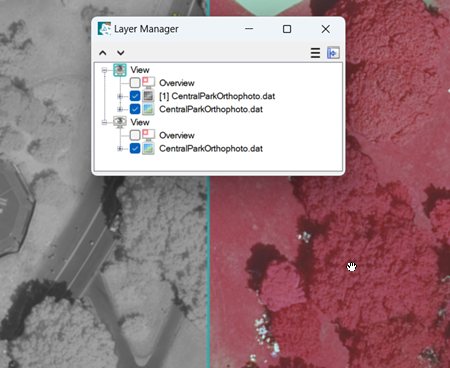
The Layer Manager shows the datasets that are displayed in the view. Since there is only one view (you will learn about multiple views later), the image layer is listed under one View category.
- Click the + button next to CentralParkOrthophoto.dat to see the bands that are used to display a true-color composite for this image.
- Click the Detach button
 in the Layer Manager to detach it from the application. It becomes a floating window that you can resize and move to a different location.
- Click the Data Manager button
 in the toolbar.
The Data Manager lists the datasets that are currently open in ENVI. For images, it also lists the available bands. Since the associated header file for this image (CentralParkOrthophoto.hdr) contains wavelength information, the Data Manager also lists the wavelengths for each band.
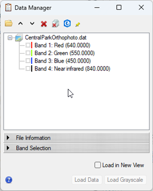
In the Data Manager, you can see that the image contains a fourth band (Band 4: Near infrared).
- Select Band 4: Near infrared and click the Load Grayscale button. The near-infrared band appears in the view, and the Layer Manager shows that a second image layer has been added to the view.
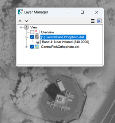
- To toggle between the two images, uncheck the [1] CentralParkOrthophoto.dat layer in the Layer Manager to hide it. Then check the layer to display it.
- Click the Cursor Value button
 in the toolbar. Red crosshairs appear in the display, along with the Cursor Value dialog.
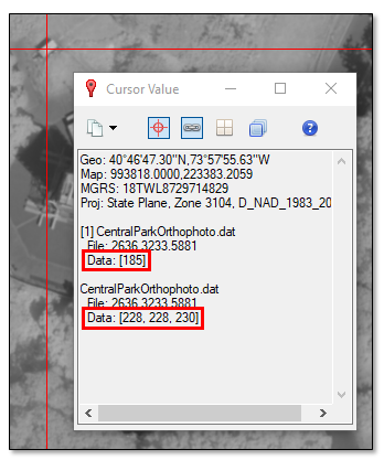
- Click anywhere in the image. The red crosshairs move to that pixel location, and the Cursor Value dialog reports the data values from the grayscale image layer and the true-color layer for that pixel.
- Close the Cursor Value dialog.
- In the Data Manager, enable the Load in New View option.
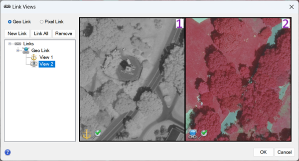
- Right-click on CentralParkOrthophoto.dat in the Data Manager and select Load CIR. A second view is added to the view, which contains a color-infrared version of the orthophoto. The colors are not real according what the human eye sees. Instead, this type of image is commonly used for discriminating between features based on the infrared response. The Layer Manager shows that a second view has been added.
Having two views provides a convenient way to compare images side-by-side. However, notice that when you zoom or pan in one view that the other view remains the same. You will need to establish a geographic link between the views.
- From the menu bar, select Views > Link Views.
-
In the Link Views dialog click the Link All button, then click OK.
Now when you zoom or pan around one view, the second view moves accordingly.
- Now is a good time to save the view layout. If you close and restart ENVI, it will not remember the layers and views that you last displayed. From the menu bar, select File > Views and Layers > Save.
- In the output file dialog, navigate to a directory where you want to save the file, and name it TwoViews.json.
- Click Save. If you close ENVI at any point in this tutorial, you can restore the views and layers from this step by selecting File > Views and Layers > Restore from the menu bar.
- Click inside of the view that contains the grayscale and true-color image layers. A cyan-colored border surrounds the view to indicate that it is the currently selected view.
- From the menu bar, select Views > One View. The color-infrared view is removed.
- In the Layer Manager, right-click on [1] CentralParkOrthophoto.dat and select Remove. Now the view only contains the true-color image.
Explore Data in More Detail
In this section you will learn more about the image data.
Image Statistics
- The orthophoto used in this tutorial is a byte image that contains data values ranging from 0 to 255 in the red, green, blue, and near-infrared bands. To confirm this, right-click on CentralParkOrthophoto.dat in the Layer Manager and select Quick Stats. Two progress dialogs appear, followed by a Statistics View dialog.
The top part shows a graphical summary of the following across all bands:
- Minimum and maximum data values (red)
- Mean data value (black)
- Standard deviation (green, centered over the mean)
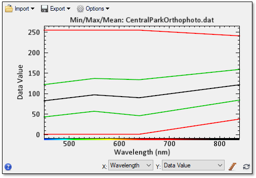
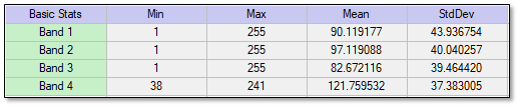
The Basic Stats section shows the actual minimum, maximum, and mean data values in each band, along with the standard deviation.
- Close the Statistics View dialog.
Spectral Profiles
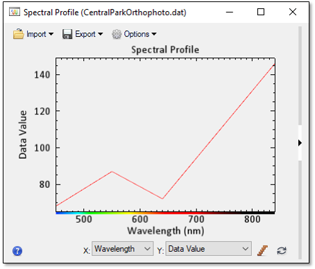
- Right-click CentralParkOrthophoto.dat in the Layer Manager and select Profiles > Spectral. Red crosshairs appear in the display, and the Spectral Profile dialog appears. A spectral profile shows the data values for a selected pixel (Y-axis) in all four bands spanning the visible to near-infrared wavelength range (X-axis).
- In the Go To field (located in the toolbar), type the values 2641p, 3588p and press the Enter key. These are pixel coordinates for a dark-green tree within the orthophoto. The "p" indicates that these are pixel coordinates, not to be confused with any map coordinates that might have the same values. The spectral profile updates to show the spectral signature of healthy, green vegetation. The curve peaks in the green wavelength region (around 550 nm), decreases in the blue and red wavelengths, and increases dramatically in the near-infrared region (above 620 nm).
- Close the Spectral Profile dialog.
Measure Distances
If an image is georeferenced to a standard map projection (as with this orthophoto), you can measure the distance between objects.
- Click the Mensuration button
 in the toolbar. Red crosshairs appear in the display, and the Cursor Value dialog appears.
- In the Go To field, enter pixel coordinates 1512.46p, 2629.02p and press the Enter key. The image centers on the first base in a softball field.
-
Click on the first base exactly where the crosshairs intersect, then click on the second base (up and to the right). A red line is drawn between the two bases.
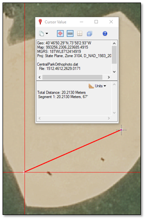
- Right-click and select Accept. The Cursor Value dialog reports the distance of the line segment (approximately 20.3 meters), along with the angle (67 degrees). The line segment becomes a polyline annotation that is added to the Layer Manager.
- Click the Units drop-down list in the Cursor Value dialog, and select US Survey Feet. What is the length of the line segment?
- Close the Cursor Value dialog.
- Right-click on New Annotation in the Layer Manager and select Remove.
- When prompted to save the changes to the new annotation, click No. The line segment is removed from the view and the Layer Manager.
Create Presentations
Next, you will learn how to modify the display properties of the image and add grid lines to the image. Steps like these are normally taken to create screen captures or full-resolution presentations that you can share with others. They do not modify the original image data in any way.
Apply a Stretch
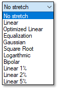
You can apply one of 10 quick stretches to the image using the Stretch Type drop-down list in the toolbar. By default, No stretch is applied to this orthophoto.
- Experiment with each option to see the effect it has on the image.
- Experiment with the Brightness, Contrast, Sharpen, and Transparency sliders in the toolbar.
Tip: The Contrast slider is only available when you choose a Linear, Equalization, Gaussian, Square Root, or Logarithmic stretch type.
You can click the Reset button next to each slider to go back to the default value. To the left of the Stretch Type drop-down list are three buttons that let you choose how the stretch is computed. By default, the Stretch on Full Extent button  is enabled, which means the selected stretch is based on the histogram of the entire image.
- Press the F11 key on your keyboard to zoom to full resolution.
- Click the Stretch on View Extent button
 in the toolbar. Now the selected stretch is only computed from the pixels that are displayed in the view.
- Pan around the image and notice how the stretch looks the same even though you are viewing a different area. You have to click the Stretch on View Extent button each time you pan around, to apply the stretch to the viewable area.
- Click the Stretch on View Extent with auto update button
 , then pan around the image. The selected stretch is automatically recomputed each time you view a different area.
- Click the Stretch on Full Extent button.
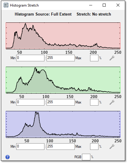
- Click the Histogram Stretch button
 in the toolbar. The Histogram Stretch dialog lets you adjust the histogram values for the red, green, and blue display bands.
- Drag the minimum and maximum vertical sliders in each histogram to see the effect the changes have on the image.
- To learn more about the different options available, click the blue help button
 in the Histogram Stretch dialog. A web browser will launch, and you will be taken to the Display Tools topic in ENVI Help.
- Close the Histogram Stretch dialog.
Tip: To cancel any changes you made in the Histogram Stretch dialog, click the Reset button  to the right of the Stretch Type drop-down list in the toolbar.
Add Grid Lines
- Click the Zoom drop-down list in the toolbar and select 12.5% (1:8).
- Click the Annotations drop-down list in the toolbar and select Grid Lines. Grid lines and labels are added to the display, but the spacing is not optimal and the labels are too small. You will modify these properties next.
- Grid line properties are displayed in the Layer panel beneath the Toolbox, in the lower-right corner of ENVI. Click in the field for the Coordinate System property and click the arrow in the field. The Select Coordinate System dialog appears.
- Type WGS 1984 in the search field of the Select Coordinate System dialog, and press the Enter key.
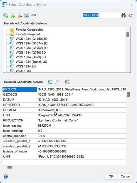
- Double-click WGS 1984 in the search results. The coordinate system changes to GCS_WGS_1984 in the Layer panel and the Select Coordinate System dialog is closed.
- Modify the following grid line properties, while leaving the remaining properties at their default values:
- X Spacing: 0.002
- Y Spacing: 0.002
- Text Font Size: 7
- Geographic Format: Degrees
- Geographic Precision: 2
- Grid Thickness: 2
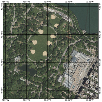
The image should look similar to the following figure:
Create a PowerPoint Presentation of the View
In the following steps you will chip the contents of the view to PowerPoint. The options under File > Chip View to will preserve any display enhancements such as brightness, stretch type, etc. It also captures any annotations that are visible in the view.
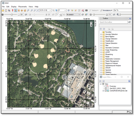
- With the zoom percentage still at 12.5%, resize the ENVI application so that the image and grid lines fill up the view and little space is left; for example:
-
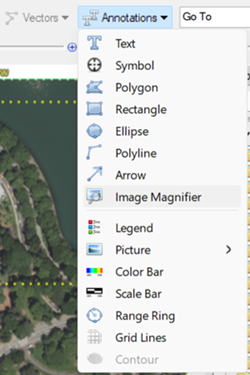
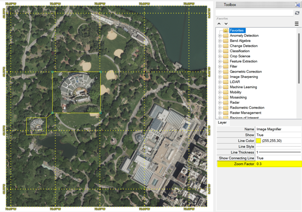
Next, you will add an annotation before you chip the view to PowerPoint. From the toolbar, click on the Annotations drop-down and select Image Magnifier.
-
Use the Image Magnifier tool to draw a box around the amphitheater. At first, the magnified image will be too large and cover much of the view.
-
In the Layer panel below the Toolbox, change the Zoom Factor property to 0.3 and press Enter.
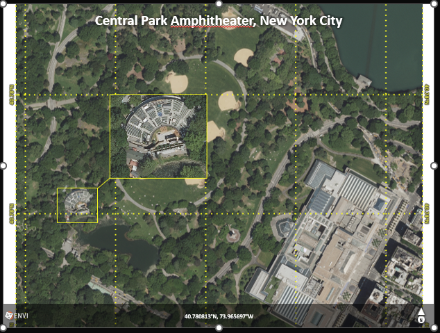
- Now, chip the view to PowerPoint. From the menu bar, select File > Chip View to > PowerPoint. The Chip to PowerPoint dialog appears.
- From the Template drop-down list, select Full Screen 4x3. This template layout emphasizes the chipped view with minimal text and graphics.
- Keep the Target Presentation selection at (Start a new presentation), and click the Chip button. The PowerPoint application opens, showing the chipped view.
-
At the top of the presentation is the heading "Title." Double-click on the heading and change the text to "Central Park Amphitheater, New York City."
- Select an output filename and location for the PowerPoint presentation.
- In ENVI, close the Chip to PowerPoint dialog, then right-click on the New Annotation layer in the Layer Manager and select Remove.
The Chip View to options are best used for taking a quick snapshot of the contents of a view; for example, to send via e-mail or to embed in a PowerPoint presentation. However, these are not ideal options when creating publication-ready images, posters, or PDF files. In these cases, you will likely want to create an output image that preserves the original resolution of the input image. You will learn how to do this next.
Export a Full-Resolution View to an Image File
The Export View to > Image File menu option exports the contents of a view, or the entire dataset extent, to an RGB 24-bit image file in ENVI or TIFF format. It preserves any annotations and image enhancements you add; however, it does not preserve the north arrow.
- Maximize the ENVI application so that it fills the screen. Or, click and drag the lower-right corner of the application to resize it however you want.
- Click the Grid layer in the Layer Manager to select it.
- Change the Text Font Size property to 18. Properties are displayed beneath the ENVI Toolbox.
- Change the Grid Thickness property to 1.
- Select the CentralParkOrthophoto.dat layer in the Layer Manager.
- Press the F11 key on your keyboard to zoom to full resolution. You do not have to pan to any particular location.
- Click the Zoom drop-down list in the toolbar and select Use Map Scale. The map scale should be 1:613.
- From the menu bar, select File > Export View to > Image File. The Export View to Image File dialog appears.
- Click the Full radio button for Output Extent. You will export the full extent of the dataset to an image file.
- In the Map Scale field, enter a denominator value of 613.
- Leave the Pixel Size and Zoom Factor fields at their default values (0.5 and 1.0).
- From the Output Format drop-down list, select TIFF.
- Select an output filename and location for the full-resolution TIFF file.
- Disable the Display result option.
- Click OK.
- Open the new TIFF file in a separate application to verify that it looks good. It should contain the entire dataset, including the grid lines. When viewed at 100% resolution, the grid line labels have a font size of 18 points.
- Right-click on the Grid layer in the Layer Manager and select Remove.
Two similar options are also available:
- File > Export View to > Geospatial PDF: This option lets you control the print resolution and page size for PDF output.
- File > Export Selected Layer to TIFF: This option exports a single image layer displayed in the view to a TIFF file. It saves the entire image extent, including any enhancements (except for sharpening) at full resolution. No other layers are retained such as annotations or vectors.
Next you will learn more about data-processing tools in ENVI.
Process Data
At the heart of ENVI is a wide variety of analytics that process image data into information used for vegetation studies, land use monitoring, defense and intelligence, and other applications. Examples of analytics include change detection, feature extraction, and classification. All of the analytics are available from the Toolbox, located on the right side of the ENVI application. The ENVI Toolbox also contains tools used for image preprocessing, raster operations, geographic positioning, and mosaicking. Tools are organized by folder according to different applications.
In this section you will run two different tools while learning about masks and regions of interest (ROIs).
Spectral Indices
Spectral indices are combinations of spectral reflectance from two or more wavelengths that indicate the relative abundance of a feature of interest. Vegetation indices are the most common type such as the Normalized Difference Vegetation Index (NDVI). To ensure the most quantitatively accurate results, the input image used for spectral indices should be in units of reflectance and corrected for atmospheric effects. You do not need to perform those steps in this tutorial. However, we provide a region of interest (ROI) file that you can use to mask out water from the image, before creating spectral index images.
- Press the F12 key on your keyboard to zoom to the full extent of the orthophoto.
- Click the Open button in the toolbar.
- Navigate to the directory where you saved the tutorial data, and select CentralParkWaterROI.xml. Click Open. Colored polygons overlay the ponds in the orthophoto.
- Type indices in the search window of the Toolbox.
- Double-click Spectral Indices. The Data Selection dialog appears.
- Click the Mask button.
- Select the Water ROI.
-
Enable the Inverse mask option.
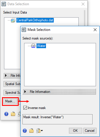
- Click OK in the Mask Selection dialog, then again in the Data Selection dialog.
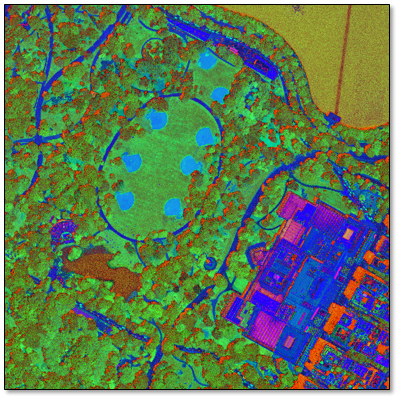
- In the Spectral Indices dialog, select Triangular Greenness Index. This index (TGI) highlights vegetation greenness in an image with red, green, and blue bands. The TGI is highly correlated with leaf chlorophyll content.
- Keep the default selection of File for Input Raster.
- Choose an output directory for the file, and name it CentralParkTGI.dat.
- Enable the Display result option.
-
Click OK. When processing is complete, the TGI image is displayed. Brighter pixels correspond to vegetation that has a light-green color in the orthophoto.
- Toggle the CentralParkTGI.dat layer on and off in the Layer Manager, to compare it with the orthophoto.
- Right-click on the CentralParkTGI.dat and Regions of Interest layers in the Layer Manager, and select Remove.
- Click the Clear Search button in the Toolbox.
Run Tasks
The ENVI application programming interface (API) contains over 200 tools called ENVITasks that you can use in a programming script. Some ENVITasks are exposed as tools in the ENVI Toolbox; for example, Spectral Indices. Others are not, such as RGB to HSI Raster and Export to PNG. However, you can still run these unexposed tasks through the ENVI user interface using the Run Task tool. The following steps provide an example.
- In the Toolbox, expand the Task Processing folder and double-click Run Task. The Run Task dialog appears.
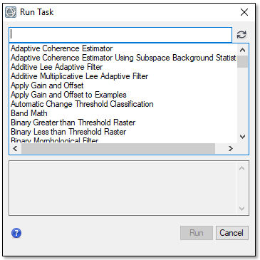
- In the Run Task dialog, type rgb in the search field.
- Select RGB to HSI Raster, and click Run. The RGB to HSI Raster dialog appears.
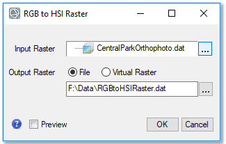
This task will create a new image that has been transformed from a red/green/blue (RGB) color space to a hue/saturation/intensity (HSI) color space. It requires an input image that only has three bands in the order of red, green, and blue. Since the orthophoto has four bands, you must define a spectral subset that only includes the first three bands.
- Click the Browse button
 next to the Input Raster field. The Data Selection dialog appears.
- Click the Spectral Subset button. The Spectral Subset dialog appears.
- Click Band 1: Red, then press the Shift key on your keyboard and select Band 3: Blue. Bands 1-3 are now selected.
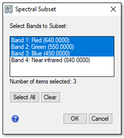
- Click OK in the Spectral Subset dialog, followed by OK in the Data Selection dialog.
- Click the Virtual Raster radio button next to Output Raster, to write the output image to memory instead of disk.
- Click OK in the RGB to HSI Raster dialog to run the task. The new HSI image appears in the view.
This concludes the tutorial. Close ENVI by selecting File > Exit from the menu bar.
Learn More
As you continue to explore ENVI, here are some resources to help you:
- ENVI supports imagery from many different sensors as well as vector formats. For a full list of data formats, see Supported Data Types.
- You can export images to different formats using the File > Save As menu. This only saves the raster data, regardless of the contents of the view.
- See Visual Programming with the ENVI Modeler to learn how to create powerful workflows in ENVI, including batch processing and running analytics in different environments.
- See the ENVI API Programming to learn how to write programming scripts that use ENVI+IDL functionality.
- See Tutorials for more exercises on using ENVI in different applications.