ENVI Crop Science contains remote sensing analytic tools for precision agriculture and agronomy. In this tutorial you will go through a typical workflow of counting crops, saving them to a shapefile, and calculating metrics to indicate their individual health. Specifically, you will do the following:
- Explore a multispectral image of a strawberry field.
- Mask out rows that contain weeds.
- Create a single-band image that enhances the strawberry plants.
- Count the strawberry plants and record their locations and sizes.
- Create a shapefile of the crop locations that were identified.
- Calculate a mean spectral index value for each plant to indicate its overall health.
- Create a presentation of the results.
This tutorial requires an installation of ENVI that includes a license for ENVI Crop Science.
Files Used in this Tutorial
Sample data files are available on our ENVI Tutorials web page. Click the "Crop Science" link in the ENVI Tutorial Data section to download the .zip file containing the data. Extract the contents to a local directory.
|
File |
Description |
|
MicaSenseStrawberries.dat
|
A sample of five-band reflectance imagery captured from the MicaSense RedEdge® UAV sensor at a height of 30 meters above the surface. The ground-sampling distance is 2 centimeters. Data courtesy of Highland Precision Ag and University of Florida.
|
|
MicaSenseStrawberries.hdr
|
Header file for above
|
|
WeedMaskROI.xml
|
ENVI region of interest (ROI) file used to mask out dirt paths and weeds.
|
Open and Explore the Image
- Start ENVI.
- Click the Open button
 in the ENVI menu bar.
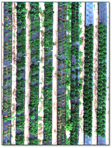
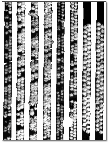
- Navigate to the location where you downloaded the tutorial data. Select the file MicaSenseStrawberries.dat and click Open. This true-color image contains several rows of green strawberry plants. Pixel values represent reflectance (0 to 100%), scaled from 0 to 1. The dark-gray areas are long strips of plastic with holes so that the strawberry plants can emerge and grow. The light brown areas are dirt paths between the planted rows.
- Click the Data Manager button
 to see the five bands listed with their respective center wavelengths. This dataset contains a Red Edge band, which measures reflectance in the red-edge wavelength region. For healthy vegetation, this region is associated with a sharp increase in the reflectance curve from red to near-infrared.
- Use the display and enhancement tools to explore the image; for example:
- Zoom in and out using the Zoom tools in the toolbar.
- Select a quick stretch option from the drop-down list in the toolbar; for example, Gaussian.
- Display a color-infrared image by right-clicking MicaSenseStrawberries.dat in the Data Manager and selecting Load CIR.
Mask Out Paths and Weeds
The case study in this tutorial involves extra steps to prepare an image for crop counting. The dirt paths contain weeds that have a similar brightness and spectral signature as the strawberry plants. These should be masked out because they will be counted along with the strawberry plants when using the Count Crops tool later. In most cases you do not need to perform these steps; however, this tutorial describes them in case you encounter similar scenarios. Please refer to the ENVI Crop Science Help for examples of simpler workflows.
- Click the Open button in the ENVI menu bar. The Open dialog appears.
- Navigate to the location where you downloaded the tutorial data. Select the file WeedMaskROI.xml and click Open. This is an ROI file that covers the dirt paths containing the weeds.
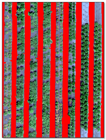
Creating an ROI to identify unwanted features is a simple process with small images such as this one. However, it is too labor-intensive when working with large images, and it cannot be done when working in a batch or enterprise environment. For this tutorial, however, an ROI file has been created for you so that you can easily mask out weeds.
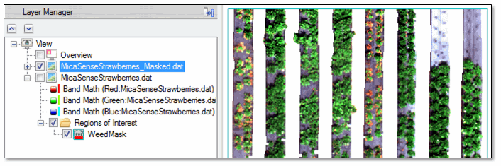
- From the ENVI menu bar, select File > Save As > Save As (ENVI, NITF, TIFF, DTED). The Data Selection dialog appears.
- Select MicaSenseStrawberries.dat. Do not click OK yet.
- Click the Mask button.
- In the Mask Selection dialog, select WeedMask.
- Enable the Inverse mask check box and click OK.
- Click OK in the Data Selection dialog. The File Save As dialog appears.
- Keep the default selection of ENVI for Output Format.
- Click the
 button next to Output Filename, and select a folder for the masked image. Name the file MicaSenseStrawberries_Masked.dat.
- Click OK. ENVI creates a mask from the ROI, and it displays the masked image in the view. The pixels in the masked regions have values of NoData and are transparent in the display. (You may need to uncheck the original true-color image in the Layer Manager to see the masked image.)
Next you will enhance the individual strawberry plants so that the crops can be accurately counted.
Enhance Crops
Later in this tutorial you will use the Count Crops tool to count the strawberry plants. That tool counts bright, circular objects in a greyscale image. You will need to create a single-band image where the strawberry plants are bright against a dark background. Here are some different options for doing this.
Spectral Indices
The quickest way to enhance crops is to create a spectral index image that highlights actively growing vegetation. However, the image must contain a near-infrared band. The image in this tutorial has a near-infrared band. Follow these steps to create a spectral index image:
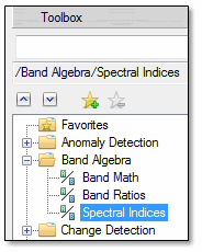
- In the ENVI Toolbox, expand the Band Algebra folder and double-click Spectral Indices.
- In the File Selection dialog, select MicaSenseStrawberries_Masked.dat and click OK. The Spectral Indices dialog appears with a list of indices that can be created from the selected image.
- Select any index from the list, then enable the Preview option to see a preview of what that index will look like.
Tip: If you zoom in or out of the image, the preview will turn off. Once you are at the preferred zoom level, enable the Preview option again.
The goal is to find an index that:
- Makes the strawberry plants bright.
- Clearly delineates each plant. Some indices such as the Normalized Difference Vegetation Index (NDVI) can over-saturate with healthy vegetation, resulting in large blurred clusters of bright pixels. This makes it difficult to distinguish individual plants from each other.
- Provides good contrast between the strawberry plants and the background.
- When you are done previewing different indices, select the Green Difference Vegetation Index (GDVI).
- Enter a filename of Strawberries_GDVI.dat for the Output Raster.
- Enable the Display result option.
- Click OK. The GDVI image is displayed:
The strawberry plants are bright, they are mostly delineated from each other, and they are highly contrasted against the background. This file will be used for the Count Crops tool later in the "Count Crops" section.
Another option is available for enhancing crops: the Enhance Crops tool. You will not use it in this tutorial, but you should be aware of its purpose.
The Enhance Crops Tool
The Enhance Crops tool (under the Crop Science folder in the Toolbox) gives you more control over isolating crops from the background while removing unwanted features. It has an option to invert the pixel values and also to set minimum and maximum pixel value thresholds. Here are some common uses:
- Healthy vegetation strongly absorbs blue and red wavelengths, so it will appear dark in blue- or red-band images. Vegetation reflects green light, but not as much as a near-infrared band. Thus, vegetation can also appear somewhat dark in a green-band image. You can use the Enhance Crops tool to invert the data values in red, green, or blue bands in order to enhance healthy vegetation. This option is useful when you only have access to RGB imagery, with no near-infrared bands.
- Remove shadows and other dark features by setting a minimum pixel value threshold. Pixels below this threshold will be set to values of NaN ("not-a-number").
- Remove features that are brighter than crops (for example, buildings or highly saturated pixels) by setting a maximum pixel threshold. Pixels above this threshold will be set to values of NaN.
Next you will learn how to use the Count Crops tool.
Count Crops
The Count Crops tool has a number of parameters that you must experiment with to obtain the best results. First, you need to know the approximate range of crop sizes in the image.
Measure the Crops
- With the GDVI image still displayed, zoom into the smallest crop you can find in the image.
- Click the Mensuration button
 in the ENVI toolbar. The Cursor Value dialog appears.
- Click on one side of the crop, then click on the opposite side. The Cursor Value dialog reports the measured distance, which should be close to 0.2 meters:
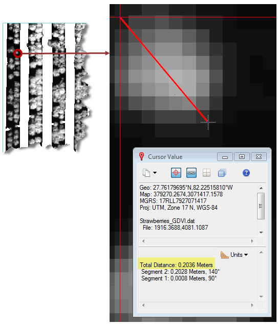
- Right-click in the display and select Clear.
- Zoom out and find one of the largest crops in the image.
- Repeat the above steps to measure that crop. It should be close to 0.4 meters, for example:

- Right-click in the display and select Clear.
- Close the Cursor Value dialog.
Count the Crops
- First, remove some rasters from the view. To do this, right-click on MicaSenseStrawberries.dat and MicaSenseStrawberries_Masked.dat in the Layer Manager and select Remove.
- In the Toolbox, expand the Crop Science folder and double-click Count Crops. The Count and Rasterize Crops dialog appears.
- Click the button next to Input Raster and select Strawberries_GDVI.dat.
- Enter a Minimum Crop Diameter value of 0.2.
- Enter a Maximum Crop Diameter value of 0.4.
- Select the Yes option for Fill Raster Crops.
- Keep all other parameters at their default values. You will use these values as starting points.
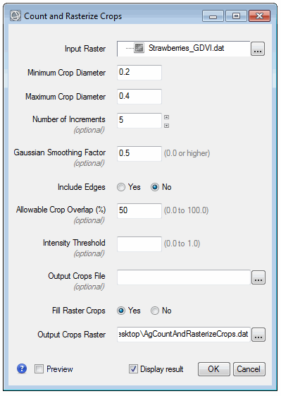
- Enable the Preview option. A preview of the crop count is displayed on top of the GDVI image. The green dots show the locations of what the tool determines are crops. The circles are sized according to what the tool determines are the actual crop sizes.
Preview the Settings and Make Adjustments
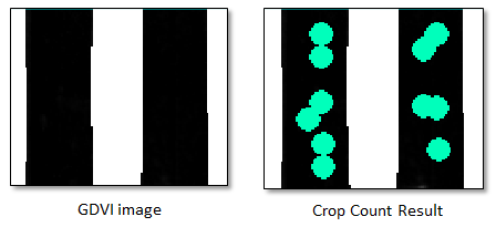
Use the Transparency slider or the View Flicker button in the toolbar to toggle between the crop count results and the underlying GDVI image. You can see that the initial result is not completely accurate. Here are some examples:
In areas of the GDVI image where no crops exist, the Count Crops tool is finding crops. This is probably because some pixels have digital number (DN) values that are close to 0 and the Count Crops tool detects them.
To fix this, experiment with the Intensity Threshold value. This parameter represents the fraction of the maximum crop intensity, below which crop detections will be removed. A higher value will remove false positives, but it might remove crops with low brightness values.
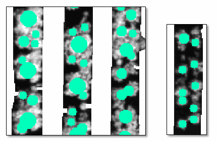
Other issues include the following, shown in the below figure:
- Multiple small crops clustered together, counted as one large crop.
- Crops not being counted.
Here are some tips for adjusting parameters to get the best results:
- Experiment with slightly different values for the Minimum Crop Diameter and Maximum Crop Diameter. The Count Crops tool works best when the diameters do not vary greatly. For example, a range of 0.2 to 0.4 meters works better than 0.1 to 0.6. If you need to expand the range of values, do so in small increments.
- Increase the Number of Increments. For example, if the Minimum Crop Diameter and Maximum Crop Diameter are 0.2 and 0.4, a value of 3 for Number of Increments means that the Count Crops tool will search for crop diameters of approximately 0.2, 0.3, and 0.4 meters. Increasing the value will make the Count Crops tool search for finer increments of crop sizes. Also, the process will take more time to run.
- Set the Include Edges parameter to Yes to count partial crops that touch the edge of the image or if you created a mask inside of the image extent (as you did earlier).
- Experiment with the Allowable Crop Overlap percentage. This is the percentage of allowable overlap between two adjacent crops before one of them is removed from consideration. The default value is 50%. In general, enter smaller values if the crops are distinctly separated from one another.
Follow these steps to continue with the crop counting process:
- Enter these parameter values, which seem to give the best results:
- Minimum Crop Diameter: 0.15
- Maximum Crop Diameter: 0.35
- Number of Increments: 30
- Gaussian Smoothing Factor: 0.5
- Include Edges: Yes
- Allowable Crop Overlap: 50
- Intensity Threshold: 0.25
- Enter a filename of OutputCrops.json for the Output Crops File.
- Set the Fill Raster Crops option to Yes.
- Enter a filename of CropCountImage.dat for the Output Crops Raster.
- Select the Display result option to display the output image when processing is complete.
- Click OK. When processing is complete, the crop count image appears in the display and Layer Manager. The final crop count is listed in the Layer Manager.
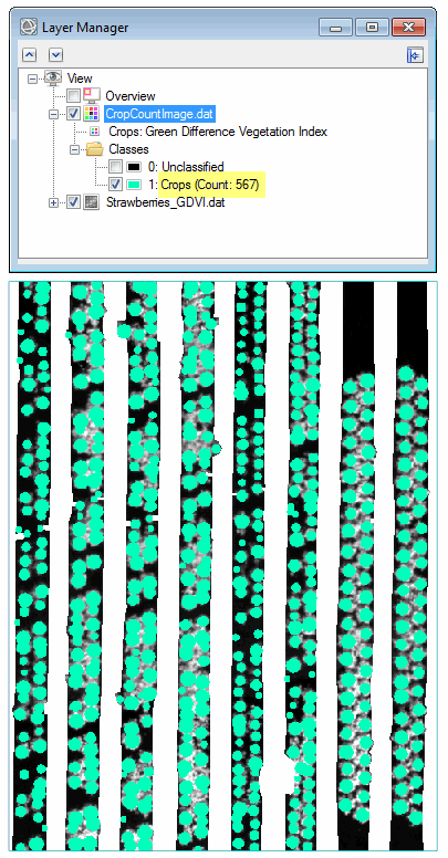
The raster form of the crop count result (CropCountImage.dat) is an ENVI classification file with two classes, Unclassified and Crops.
The crop count file is a JSON-formatted text file. In the next section you will convert this to a shapefile.
Convert Crops to a Shapefile
The crops file is in JSON text format. It contains the X,Y pixel locations of each counted crop. If you were to open OutputCrops.json in a text editor, you would see the following:
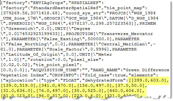
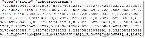
Scrolling down further in this file, you would see the radius of each detected crop:
Converting the JSON file to a shapefile will make the crop count result easier to work with. The crop locations and radii will be included in the shapefile attribute table, plus you can add more custom attributes as needed.
Follow these steps:
- In the Toolbox, double-click Convert Crops To Shapefile.
- Click the button next to Input Crops, and select OutputCrops.json.
- Enter an output filename of OutputCrops.shp in the Output Vector field.
- Enable the Display result option.
- Click OK. When processing is complete, the shapefile is added to the display and Layer Manager.
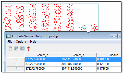
- Right-click on OutputCrops.shp in the Layer Manager, and select View/Edit Attributes. The Attribute Viewer lists the center X,Y location for each crop, along with its radius.
- Click on an item in the display to highlight its corresponding record in the Attribute Viewer; for example:
- Close the Attribute Viewer, and uncheck OutputCrops.shp in the Layer Manager to hide it.
- Right-click in the display and select Clear Selections.
Now that you know the crop locations, you can calculate some metrics to determine their overall health. You will do this in the next section.
Calculate Crop Metrics
In this section you learn how to use the Calculate Crop Metrics with Spectral Index tool. This tool lets you create a classification image showing the relative mean values of crops, or a greyscale image showing their actual means.
Create an NDVI Classification Image
- In the Toolbox, double-click Calculate Crop Metrics with Spectral Index.
- In the File Selection dialog, select MicaSenseStrawberries_Masked.dat. Click Open, then OK. The crop metrics will be calculated from the original multispectral image, but only at the selected X,Y locations recorded in the crops file (OutputCrops.json).
- Click the button next to Input Crops, and select OutputCrops.json.
- From the Spectral Index drop-down list, select Normalized Difference Vegetation Index. Although you can choose any supported vegetation index, NDVI is the most common and recognizable index associated with vegetation health.
- Leave the default selection of Crop Mean for Output Metric.
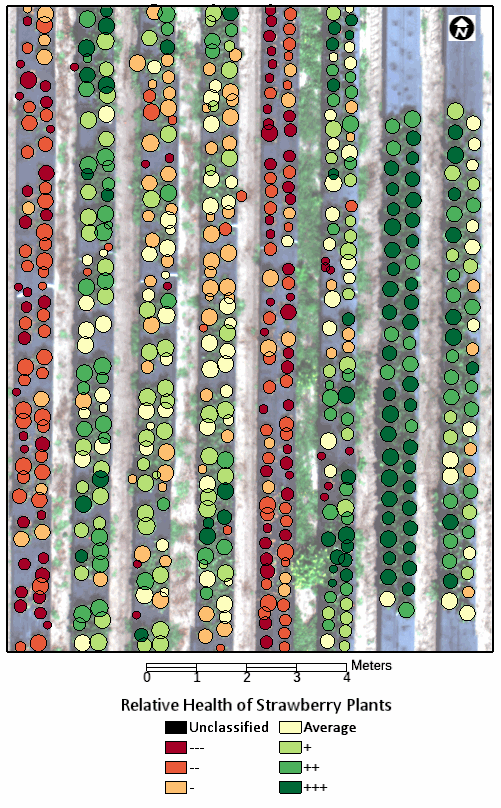
- For this first exercise, you will create a classification raster of relative NDVI means. Select the Yes option for Create Classification Raster.
- Enter an output filename of StrawberryRelativeNDVI.dat.
- Leave the Output Crops File field blank.
- Enable the Display result option.
- Click OK. When processing is complete, the classification image appears in the display:
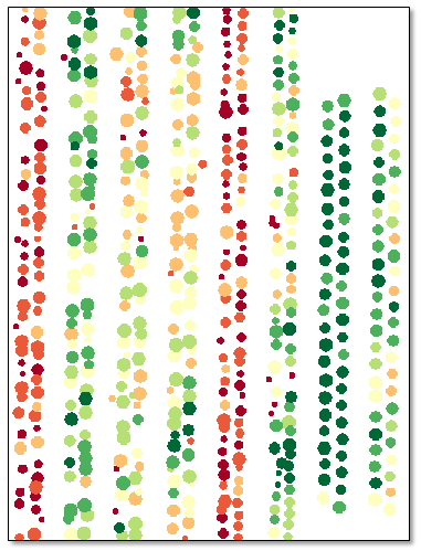
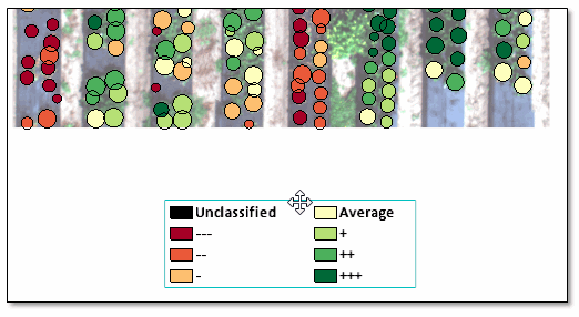
The Layer Manager shows the class legend. The classes represent relative NDVI means with respect to the entire image. For example, a dark green polygon corresponds to a crop with a higher mean NDVI value than light-green, yellow, and red polygons.
Next, you will run the same tool again but create a different type of image.
Create a Greyscale Image of NDVI Means
In this exercise you will create an image that shows actual mean NDVI values for each strawberry plant.
- In the Toolbox, double-click Calculate Crop Metrics with Spectral Index.
- In the File Selection dialog, select MicaSenseStrawberries_Masked.dat. Click OK.
- From the Spectral Index drop-down list, select Normalized Difference Vegetation Index.
- Click the button next to Input Crops, and select OutputCrops.json.
- Leave the default selection of Crop Mean for Output Metric.
- Select the No option for Create Classification Raster.
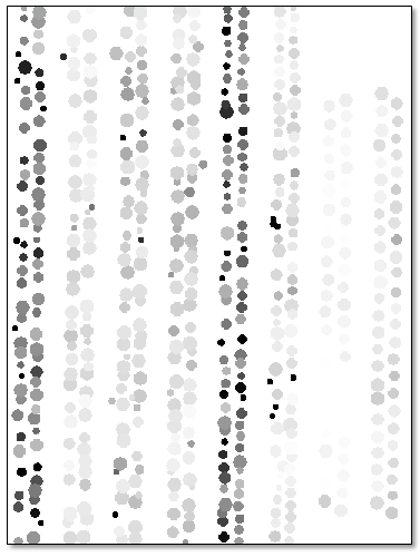
- Enter an output filename of StrawberryNDVIMeans.dat.
- Leave the Output Crops File field blank.
- Enable the Display result option.
- Click OK. When processing is complete, a greyscale image appears in the display:
- Click the Cursor Value button
 in the main toolbar.
- Click on any grey circle. The Cursor Value dialog reports the mean NDVI value for that strawberry plant (under the StrawberryNDVIMeans.dat layer); for example:
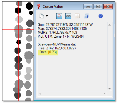
These metrics and this type of image may be helpful for agronomists who want a more detailed analysis of crop health in a given area.
Optional: Create a Raster Color Slice of the NDVI Means
Now that you have a greyscale raster of NDVI means, you can create a classification image of those values. Follow these steps:
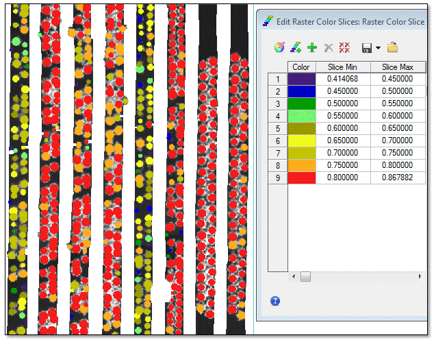
- Right-click on the StrawberryNDVIMeans.dat layer in the Layer Manager and select New Raster Color Slice.
- In the File Selection dialog, select Crop Mean: Normalized Difference Vegetation Index and click OK. ENVI determines the range of NDVI values and splits them into categories by color, ranging from purple (0.414) to red (0.868). You can accept these color slices, or create your own. The following image shows an example of a custom color slice, overlaying the GDVI image:
- Click the Export Color Slices button
 in the Edit Raster Color Slices dialog, and select Export as Class Image.
- In the Export Color Slices to Class Image dialog, enter an output filename of NDVIColorSlices.dat and click OK.
- Click OK in the Edit Raster Color Slices dialog.
- Close the Cursor Value dialog.
- To prepare for the next section, right-click on the following layers and select Remove:
- Raster Color Slice
- StrawberryNDVIMeans.dat
- MicaSenseStrawberries_Masked.dat
- Strawberries_GDVI.dat
Present the Results
In this section you will create a presentation of the relative NDVI means by adding some annotations. You will then export the presentation to a GeoTIFF file.
- Click the Open button in the toolbar and select MicaSenseStrawberries.dat.
- In the Layer Manager, drag the StrawberryRelativeNDVI.dat layer above MicaSenseStrawberries.dat. The relative NDVI classification image now overlays the multispectral image.
Display Crop Outlines
The next few steps will help create a better visualization of the strawberry plants that were counted with the Count Crops tool. You will use the crops shapefile to draw outlines of each crop location.
- In the Layer Manager, drag the OutputCrops.shp layer above the other layers. Also, select its check box to display it.
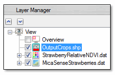
- Right-click OutputCrops.shp in the Layer Manager and select Properties.
- In the Vector Properties dialog, set the Line Color to black and the Line Thickness to 1. Click OK. The following figure shows how the different data layers appear:
Add Annotations
- In the Layer Manager, select the MicaSenseStrawberries.dat layer to make it the active layer.
- Zoom to 100%.
- From the ENVI menu bar, select File > Preferences.
- On the left side of the Preferences dialog, select North Arrow.
- Click in the Font field and select ESRI North using the drop-down arrow that appears.
- Click the Symbol field, then click the drop-down arrow that appears. Select a different north arrow symbol and click OK.
- Click OK in the Preferences dialog.
- Right-click on the View layer in the Layer Manager and select New > Annotation Layer.
- In the Create New Annotation Layer dialog, change the Layer Name to Strawberry Annotations.
- Select StrawberryRelativeNDVI.dat in the Source Data list and click OK.
- With Strawberry Annotations selected in the Layer Manager, click the Annotations drop-down list in the menu bar and select Legend.
- Click in the display near the bottom of the image.
- In the File Selection dialog, select StrawberryRelativeNDVI.dat and click OK. A classification legend is displayed.
- Double-click the Legend layer in the Layer Manager to display the Properties dialog.
- Change these properties as desired: Legend Columns, Font Name, Font Style, and Font Size. You can also edit the class names if desired.
- To move the legend annotation, select Legend in the Layer Manager. Move your cursor over the legend until an icon with four arrows appears. Then move the legend as needed.
- Add the following annotation types using the Annotations drop-down list: Text, Scale Bar, and Rectangle (to create a border around the image or classification legend). Then modify their properties as desired.
- Right-click on the Strawberry Annotations layer in the Layer Manager and select Save As.
- Accept the default filename of Strawberry_Annotations.anz and click Save.
Here is an example of a simple layout:
Save the View Layout
You should save the layout that you prepared in case you need to modify it later. The layout includes the images and annotations that are listed in the Layer Manager. From the ENVI menu bar, select File > Views & Layers > Save. Enter an output filename of StrawberryHealthMap.json and click Save.
Save the Layout to a GeoTIFF File
Saving the map layout to a GeoTIFF file will preserve the images and annotations. An Export View to Geospatial PDF option is also available, but it only saves image layers (not annotations). Follow these steps:
- From the ENVI menu bar, select File > Export View to > Image File. The Export View to Image File dialog appears.
- Select the Full option for Output Extent.
- Leave the Map Scale, Pixel Size, and Zoom Factor at their default values.
- From the Output Format drop-down list, select TIFF.
- Enter an output Filename of StrawberryHealthMap.tif.
- Enable the Display result option.
- Click OK.
To change the scale of the layout, you can further experiment with the annotation properties (especially font sizes) as well as different Map Scale, Pixel Size, and Zoom Factor values in the Export View to Image File dialog.
Another option that you may find useful is File > Chip View To > Powerpoint. This and other Chip View To options essentially create screen captures of your view.
This concludes the Crop Counting and Metrics tutorial. For more information on ENVI Crop Science, refer to the ENVI Crop Science section in ENVI Help.