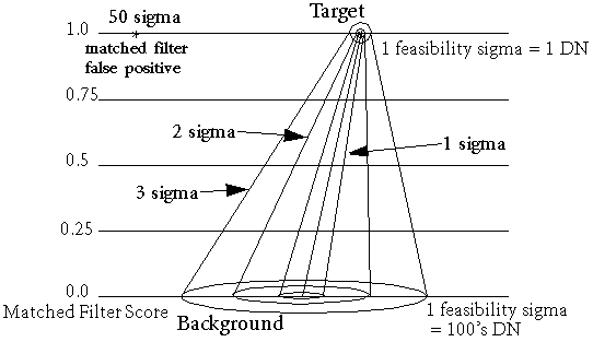
Use Mixture Tuned Matched Filtering (MTMF) to perform Matched Filtering (MF) and to add an infeasibility image to the results. The infeasibility image is used to reduce the number of false positives that are sometimes found when using MF. Pixels with a high infeasibility are likely to be MF false positives. Correctly mapped pixels will have an MF score above the background distribution around zero and a low infeasibility value. The infeasibility values are in noise sigma units that vary in DN scale with an MF score (see the following figure). For additional information, see Mixture Tuned Matched Filtering Results.
MTMF requires an MNF transform input file, or other data with isotropic, unit variance noise.
You can write a script to perform MTMF using the MixtureTunedMatchedFilter task.

Note: See Spectral Hourglass Workflow for instructions on the ENVI hourglass processing flow, including MNF transforms and MTMF, to find and map image spectral endmembers from hyperspectral or multispectral data.
- From the Toolbox, select Spectral > Mapping Methods > Mixture Tuned Matched Filtering. The Mixture Tuned Matched Filter Input File dialog appears.
- Select the input MNF file and perform optional spatial and spectral subsetting, then click OK. The Endmember Collection:Mixture Tuned MF dialog appears.
- Import the spectra to match. See Import Spectra for details.
The spectra must be in MNF space. You can calculate the spectra from ROIs in the MNF input file or transform them into MNF space.
Note: The input spectra must be pure and spectrally extreme endmembers, for the MTMF to be interpretable. You can identify these types of endmembers using the Pixel Purity Index (PPI) and n-Dimensional Visualizer.
- Click Apply. The Mixture Tuned Matched Filter Parameters dialog appears.
- Use the toggle button to select Compute New Covariance Stats and enter an output statistics filename, or toggle to Use Existing Stats File.
- If you selected Compute New Covariance Stats: To remove anomalous pixels before calculating background statistics, enable the Subspace Background check box. Then, specify in the Background Threshold field the fraction of the background in the anomalous image to use for calculating the subspace background statistics. The threshold range is 0.500 to 1.000 (the entire image).
- Select output to File or Memory.
- From the Output Data Type drop-down list, select Byte or Floating Point.
- If you select Byte, enter a Min and Max stretch value.
- Click OK.
- If you selected Use Existing Stats File, select the statistics file that corresponds to the input data file when the Input File dialog appears. This statistics file must contain both the mean and covariance statistics for the input data.
Mixture Tuned Matched Filtering Results
The output from MTMF is a set of rule images corresponding to both the MF score and the infeasibility score for each pixel compared to each endmember spectrum (two rule images per endmember). The MF floating-point results help estimate the relative degree of match to the reference spectrum and the approximate sub-pixel abundance, where 1.0 is a perfect match. The infeasibility results are in noise sigma units and indicate the feasibility of the MF result. Correctly mapped pixels have an MF score above the background distribution, which has some noise-limited spread around zero, and a low infeasibility value.
You can use a 2D scatter plot to identify the pixels with low infeasibilities and high MF scores. Use interactive stretching to stretch the upper tail of the histogram when viewing the MF resulting bands to show only pixels containing the target material.
- In the Layer Manager, select an MF Score image, click the Gray Scale radio button, and click Load Band.
- From the menu bar, select Display > 2D Scatter Plot.
- Select an MF Score image from the X Band list, and select the corresponding Infeasibility image from the Y Band list.
- Pixels with high MF scores and high infeasibility are probably false alarms and should be rejected. Ideally, you should see a horizontal arm of true detections across the bottom of the scatter plot. You can retrieve reliable sub-pixel abundance values from the MF scores for low-infeasibility pixels.